Easy Bayesian linear modeling
STA602 at Duke University
Exercise 2
Examining the output
- Did
stan_glmdo what we think it did? Did the Markov chain converge? Which parameters, if any, have a 90% credible interval that covers 0?
Notice sample: 1000 since half get thrown away by stan and is called “burn-in” i.e. a period that the chain spends reaching the target distribution gets discarded.
Model Info:
 function:     stan_glm
 family:       binomial [logit]
 formula:      type ~ .
 algorithm:    sampling
 sample:       1000 (posterior sample size)
 priors:       see help('prior_summary')
 observations: 3680
 predictors:   58

Estimates:
                    mean   sd    10%   50%   90%
(Intercept)        -3.9    0.5  -4.5  -3.9  -3.4
make               -0.1    0.1  -0.2  -0.1   0.0
address            -0.2    0.1  -0.4  -0.2  -0.1
all                 0.1    0.1   0.0   0.1   0.1
num3d               0.9    0.7   0.2   0.7   1.7
our                 0.4    0.1   0.3   0.4   0.5
over                0.2    0.1   0.1   0.2   0.3
remove              0.9    0.1   0.7   0.9   1.1
internet            0.2    0.1   0.1   0.2   0.3
order               0.1    0.1   0.0   0.1   0.2
mail                0.1    0.0   0.0   0.1   0.1
receive             0.0    0.1  -0.1   0.0   0.0
will               -0.2    0.1  -0.3  -0.2  -0.1
people             -0.1    0.1  -0.1   0.0   0.0
report              0.0    0.1  -0.1   0.0   0.1
addresses           0.3    0.2   0.1   0.3   0.5
free                1.0    0.1   0.8   1.0   1.1
business            0.5    0.1   0.3   0.5   0.6
email               0.1    0.1   0.0   0.1   0.2
you                 0.1    0.1   0.0   0.1   0.2
credit              0.6    0.2   0.3   0.6   0.9
your                0.3    0.1   0.2   0.3   0.4
font                0.2    0.2   0.1   0.2   0.4
num000              0.7    0.2   0.5   0.7   0.9
money               0.2    0.1   0.1   0.2   0.3
hp                 -3.1    0.5  -3.8  -3.1  -2.5
hpl                -1.0    0.4  -1.5  -1.0  -0.5
george             -8.5    1.8 -10.9  -8.5  -6.3
num650              0.2    0.1   0.1   0.2   0.4
lab                -1.1    0.5  -1.8  -1.0  -0.5
labs               -0.1    0.1  -0.3  -0.1   0.0
telnet             -0.3    0.3  -0.8  -0.3   0.0
num857             -0.2    0.6  -1.0  -0.2   0.4
data               -0.7    0.2  -1.0  -0.7  -0.5
num415             -0.6    0.8  -1.7  -0.5   0.2
num85              -0.8    0.4  -1.3  -0.8  -0.3
technology          0.4    0.1   0.2   0.4   0.6
num1999             0.0    0.1  -0.1   0.0   0.1
parts              -0.2    0.1  -0.4  -0.2  -0.1
pm                 -0.4    0.2  -0.6  -0.4  -0.2
direct             -0.2    0.1  -0.3  -0.1   0.0
cs                 -1.4    0.8  -2.4  -1.2  -0.5
meeting            -1.5    0.5  -2.2  -1.5  -1.0
original           -0.4    0.2  -0.8  -0.4  -0.1
project            -1.3    0.4  -1.8  -1.3  -0.8
re                 -0.7    0.2  -0.9  -0.7  -0.5
edu                -1.5    0.3  -1.9  -1.5  -1.1
table              -0.3    0.1  -0.5  -0.3  -0.1
conference         -1.1    0.4  -1.7  -1.1  -0.6
charSemicolon      -0.3    0.1  -0.5  -0.3  -0.2
charRoundbracket   -0.1    0.1  -0.2  -0.1   0.0
charSquarebracket  -0.1    0.1  -0.3  -0.1   0.0
charExclamation     0.2    0.1   0.2   0.2   0.3
charDollar          1.2    0.2   1.0   1.3   1.5
charHash            0.7    0.4   0.2   0.7   1.2
capitalAve          0.0    0.3  -0.3   0.0   0.4
capitalLong         0.9    0.4   0.4   0.8   1.3
capitalTotal        0.7    0.1   0.5   0.7   0.8

Fit Diagnostics:
           mean   sd   10%   50%   90%
mean_PPD 0.4    0.0  0.4   0.4   0.4

The mean_ppd is the sample average posterior predictive distribution of the outcome variable (for details see help('summary.stanreg')).

MCMC diagnostics
                  mcse Rhat n_eff
(Intercept)       0.0  1.0   740
make              0.0  1.0  1161
address           0.0  1.0  1156
all               0.0  1.0   907
num3d             0.0  1.0   958
our               0.0  1.0   973
over              0.0  1.0  1022
remove            0.0  1.0   909
internet          0.0  1.0  1188
order             0.0  1.0  1064
mail              0.0  1.0  1022
receive           0.0  1.0  1171
will              0.0  1.0  1022
people            0.0  1.0  1307
report            0.0  1.0   935
addresses         0.0  1.0  1115
free              0.0  1.0   830
business          0.0  1.0  1059
email             0.0  1.0   895
you               0.0  1.0  1026
credit            0.0  1.0  1328
your              0.0  1.0  1077
font              0.0  1.0  1226
num000            0.0  1.0  1124
money             0.0  1.0   910
hp                0.0  1.0  1161
hpl               0.0  1.0  1422
george            0.1  1.0   779
num650            0.0  1.0  1017
lab               0.0  1.0  1477
labs              0.0  1.0  1317
telnet            0.0  1.0  1002
num857            0.0  1.0  1388
data              0.0  1.0  1265
num415            0.0  1.0  1427
num85             0.0  1.0  1247
technology        0.0  1.0  1021
num1999           0.0  1.0   834
parts             0.0  1.0  1227
pm                0.0  1.0  1135
direct            0.0  1.0   793
cs                0.0  1.0  1293
meeting           0.0  1.0  1547
original          0.0  1.0  1805
project           0.0  1.0  1432
re                0.0  1.0  1027
edu               0.0  1.0  1048
table             0.0  1.0  1082
conference        0.0  1.0  1492
charSemicolon     0.0  1.0  1308
charRoundbracket  0.0  1.0   906
charSquarebracket 0.0  1.0  1286
charExclamation   0.0  1.0  1070
charDollar        0.0  1.0  1147
charHash          0.0  1.0  1111
capitalAve        0.0  1.0  1165
capitalLong       0.0  1.0  1421
capitalTotal      0.0  1.0  1312
mean_PPD          0.0  1.0   909
log-posterior     0.5  1.0   338

For each parameter, mcse is Monte Carlo standard error, n_eff is a crude measure of effective sample size, and Rhat is the potential scale reduction factor on split chains (at convergence Rhat=1).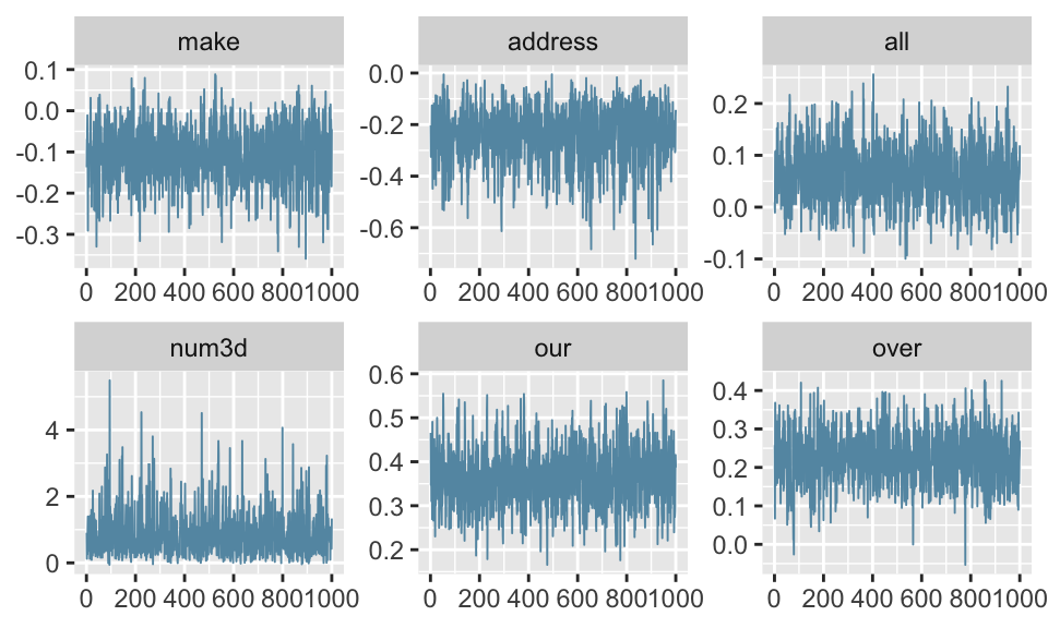
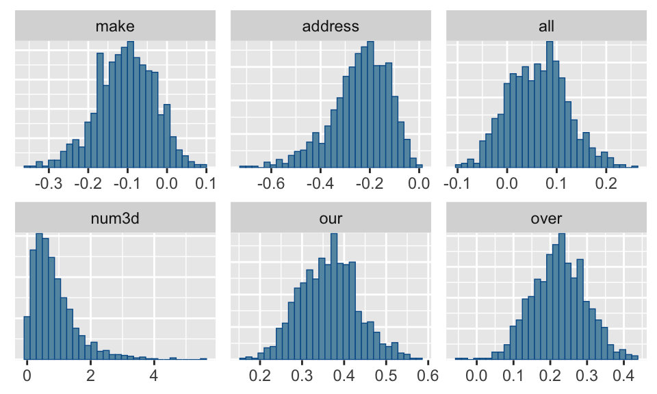
To plot specific parameters, use the arguemnt pars, e.g.
mcmc_trace(fit1, pars = c("internet", "george")mcmc_hist(fit1, pars = "make")
To read more about bayesplot functionality, see https://mc-stan.org/bayesplot/articles/plotting-mcmc-draws.html
chain_draws = as_draws(fit1)
chain_draws$george[1:5] # first 5 samples of the first chain run by stan
[1] -8.657706 -8.058416 -7.542682 -5.875524 -10.805427- try the following command:
View(chain_draws)
Report posterior mean, posterior median and 90% posterior CI.
posteriorMean = apply(chain_draws, 2, mean)
posteriorMedian = fit1$coefficients
posteriorCI = posterior_interval(fit1, prob = 0.9)
cbind(posteriorMean, posteriorMedian, posteriorCI)
posteriorMean posteriorMedian 5% 95%
(Intercept) -3.92819676 -3.89842329 -4.688486640 -3.214996079
make -0.10511093 -0.10291579 -0.234925630 0.007473911
address -0.23994990 -0.22496984 -0.459838123 -0.079085239
all 0.06181680 0.06204777 -0.032348802 0.162371165
num3d 0.86239227 0.69068831 0.094477008 2.262920466
our 0.36326097 0.36517847 0.252660614 0.482222431
over 0.22388788 0.22526813 0.104903413 0.345376589
remove 0.89046939 0.88519560 0.660560624 1.124715173
internet 0.19219955 0.18873972 0.084482068 0.313373050
order 0.14088547 0.14175852 0.022540540 0.262790934
mail 0.07091792 0.07049483 -0.004812217 0.148380741
receive -0.04641076 -0.04704090 -0.155648064 0.056349226
will -0.19669579 -0.19506749 -0.323302246 -0.079179801
people -0.05080340 -0.04939546 -0.170276558 0.067469609
report -0.01152332 -0.01105396 -0.102076144 0.078218538
addresses 0.27381609 0.26410052 0.016663808 0.554382803
free 0.95909363 0.95496752 0.738679361 1.184988932
business 0.46684266 0.46497563 0.276894271 0.663670058
email 0.10488455 0.10024984 0.001909845 0.222419640
you 0.10146793 0.10210904 -0.005066755 0.212057793
credit 0.60260737 0.58770051 0.245466733 1.011651069
your 0.29510195 0.29496631 0.185160138 0.408134909
font 0.23712284 0.22816521 0.014405002 0.514370136
num000 0.71052738 0.69647322 0.470113449 0.973663603
money 0.20621767 0.19864778 0.101091758 0.340661983
hp -3.12311740 -3.10880324 -4.016671505 -2.304686191
hpl -1.03485238 -1.03298227 -1.697441864 -0.401214421
george -8.54020532 -8.47338329 -11.651960267 -5.719147532
num650 0.23079106 0.22722517 0.066179720 0.417323354
lab -1.06217022 -0.98480464 -2.007243002 -0.334531315
labs -0.12552567 -0.11162875 -0.398538494 0.091786582
telnet -0.34336793 -0.26439840 -0.971412117 0.026123689
num857 -0.24559769 -0.15437261 -1.410789083 0.608907729
data -0.73133589 -0.71699338 -1.108487928 -0.382954624
num415 -0.64101304 -0.47534569 -2.093090996 0.285482781
num85 -0.79569146 -0.76847847 -1.439452875 -0.215331103
technology 0.39271940 0.38676108 0.173703662 0.625821033
num1999 -0.01626319 -0.01501346 -0.146351106 0.113311375
parts -0.19387536 -0.17594695 -0.420298806 -0.034525634
pm -0.36307678 -0.35286882 -0.654982493 -0.099008434
direct -0.16079193 -0.14842066 -0.405108058 0.023707001
cs -1.35347826 -1.21771081 -2.748096259 -0.377142268
meeting -1.54394154 -1.48634297 -2.451147222 -0.853955898
original -0.44492327 -0.43068267 -0.889558420 -0.068304526
project -1.27091449 -1.25700373 -1.901896255 -0.691331691
re -0.68897480 -0.68667471 -0.941480034 -0.439694059
edu -1.52342346 -1.51146322 -2.056088445 -1.041884151
table -0.27888780 -0.25736694 -0.549891396 -0.077155657
conference -1.10733935 -1.06265166 -1.864536810 -0.460671052
charSemicolon -0.32588657 -0.31416332 -0.514101364 -0.166688438
charRoundbracket -0.08698799 -0.08292353 -0.212643020 0.023441788
charSquarebracket -0.14980893 -0.13280261 -0.342135625 -0.004178006
charExclamation 0.23238206 0.22752584 0.137507390 0.351658871
charDollar 1.24928427 1.25351495 0.944702156 1.558125382
charHash 0.71795213 0.70213467 0.122922001 1.368832748
capitalAve -0.01033156 -0.03262611 -0.401092859 0.470713740
capitalLong 0.85197631 0.82214223 0.303300262 1.493571408
capitalTotal 0.67337732 0.67245181 0.471182694 0.893198052