Maximum likelihood estimator

STA602 at Duke University

Background: likelihoods

Example: normal likelihood

Let \(X\) be the resting heart rate (RHR) in beats per minute of a student in this class.

Assume RHR is normally distributed with some mean \(\mu\) and standard deviation \(8\).

\[ \textbf{Data-generative model: } X_i \overset{\mathrm{iid}}{\sim} N(\mu, 64) \]

If we observe three student heart rates, {75, 58, 68} then our likelihood

\[L(\mu) = f_x(75 |\mu) \cdot f_x(58|\mu) \cdot f_x(68|\mu).\]

That is, the joint density function of the observed data, viewed as a function of the parameter.

Important

The likelihood itself is not a density function. The integral with respect to the parameter does not need to equal 1.

Visualizing the likelihood

\[L(\mu) = f_x(75 |\mu) \cdot f_x(58|\mu) \cdot f_x(68|\mu).\]

• data
• likelihood function
• plot
• plot code

x = c(75, 58, 68)

L = function(mu, x) {
  stopifnot(is.numeric(x))
  n = length(x)
  likelihood = 1
  for(i in 1:n){
    likelihood = likelihood * dnorm(x[i], mean = mu, sd = 8)
  }
  return(likelihood)
}

ggplot() +
  xlim(c(50, 83)) +
  geom_function(fun = L, args = list(x = x)) +
  theme_bw() +
  labs(x = expression(mu), y = "likelihood") + 
  geom_vline(xintercept = 67, color = 'red')

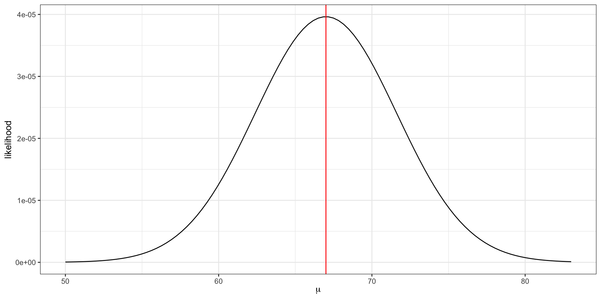
The maximum likelihood estimate \(\hat{\mu} = \frac{75 + 58 + 68}{3} = 67\).

The maximum likelihood estimate is the parameter value that maximizes the likelihood function.

The log-likelihood

Notice how small the y-axis is on the previous slide. What happens to the scale of the likelihood as we add additional data points?

\[ L(\mu) = \prod_{i = 1}^{n} f_x(x_i |\mu) \]

Since densities often evaluate between 0 and 1, multiplying many together (as we usually do in likelihoods) can quickly result in floating point underflow. That is, numbers smaller than the computer can actually represent in memory.

• Note: sometimes densities evaluate to greater than 1 (e.g. dnorm(0, 0, 0.001)) and multiplying several together can result in overflow.

log to the rescue!

• log is a monotonic function, i.e. \(x > y\) implies \(\log(x) > \log(y)\), because of this the maximum of \(f\) is the same as the maximum of \(\log f\).

• additionally, log turns products into sums

in practice, we always work with the log-likelihood,

\[ \log L(\mu) = \sum_{i = 1}^n \log f_x(x_i | \mu). \]

MLE

Maximum likelihood estimation (MLE)

How did we know to take the average of the values to find the maximum likelihood estimator \(\hat{\mu}\)?

From calculus, we know that to maximize a function, we need to find where the slope equals zero (technically, to ensure we find some maxima and not a minima we need to also check that the second derivative is negative).

Example: normal likelihood

For the normal likelihood example on the previous slide, we can see visually that the function is concave.

To find the maximum,

\[ \begin{aligned} \frac{d}{d\mu} \log L(\mu) &= \sum_{i}\frac{d}{d\mu} \log f_x(x_i |\mu)\\ &= \sum_{i}\frac{d}{d\mu} \left[ -\frac{1}{2} \log (2 \pi \sigma^2) - \frac{1}{2\sigma^2} (x_i - \mu)^2 \right]\\ &= \sum_i \frac{1}{\sigma^2} (x_i - \mu) \end{aligned} \]

Setting the derivative equal to zero,

\[ \begin{aligned} \sum_i \left[ x_i - \hat{\mu} \right] &= 0\\ n \hat{\mu} &= \sum_i x_i\\ \hat{\mu} &= \bar{x} \end{aligned} \]

Exercise: binomial MLE

Let \(Y_1, Y_2, \ldots, Y_n \sim \text{iid } \text{binary}(\theta)\). Here \(\theta\) is the probability of a success, i.e. \(prob(Y_i = 1)\).

• Note: a “binary” distribution is equivalent to a “Bernoulli” distribution. Your book calls it “binary”, so we will as well for consistency.

1. Write down the likelihood, \(p(y_1, \ldots, y_n | \theta)\).

2. Write down the log-likelihood.

3. Compute \(\hat{\theta}_{MLE} = \text{argmax}_{\theta}~ \log p(y_1, \ldots, y_n | \theta)\)

Solution

• solution 1
• solution 2
• solution 3

\[ \begin{aligned} p(y_1, \ldots, y_n | \theta) &= \prod_{i=1}^n p(y_i | \theta)\\ &= \theta^{y_i}(1-\theta)^{1-y_i}\\ &= \theta^{\sum {y_i}}(1-\theta)^{n - \sum y_i} \end{aligned} \]

\[ \log \left(\theta^{\sum {y_i}}(1-\theta)^{n - \sum y_i} \right) = n \bar{y} \log \theta + n(1-\bar{y}) \log(1 - \theta) \]

where \(\bar{y} = \frac{1}{n} \sum_{i=1}^n y_i\).

Take the derivative

\[ \begin{aligned} \frac{d}{d\theta} \log p(y_1, \ldots, y_n | \theta) &= \frac{n\bar{y}}{\theta} - \frac{n - n\bar{y}}{1- \theta} \end{aligned} \]

and set equal to 0. After simplifying,

\[ \hat{\theta}_{MLE} = \bar{y} \]