Normal modeling &
Bayesian estimators

STA602 at Duke University

Normal model

Exercise

Libraries used:

library(tidyverse)
library(latex2exp)

Data

bass = read_csv("https://sta360-sp25.github.io/data/bass.csv")

glimpse(bass)

Rows: 171
Columns: 5
$ river   <dbl> 0, 0, 0, 0, 0, 0, 0, 0, 0, 0, 0, 0, 0, 0, 0, 0, 0, 0, 0, 0, 0,…
$ station <dbl> 0, 0, 0, 0, 0, 0, 0, 0, 0, 0, 1, 1, 1, 1, 1, 1, 1, 1, 1, 1, 1,…
$ length  <dbl> 47.0, 48.7, 55.7, 45.2, 44.7, 43.8, 38.5, 45.8, 44.0, 40.4, 47…
$ weight  <dbl> 1.616, 1.862, 2.855, 1.199, 1.320, 1.225, 0.870, 1.455, 1.220,…
$ mercury <dbl> 1.60, 1.50, 1.70, 0.73, 0.56, 0.51, 0.48, 0.95, 1.40, 0.50, 0.…

Mercury, is a naturally occurring element that can have toxic effects on the nervous, digestive and immune systems of humans. Bass from the Waccamaw and Lumber Rivers (NC) were caught randomly, weighed, and measured. In addition, a filet from each fish caught was sent to the lab so that the tissue concentration of mercury could be determined for each fish. Each fish caught corresponds to a single row of the data frame. Today we will examine two columns from the data set: mercury (concentration of mercury in ppm) and weight (weight of the fish in kg). We’ll model the mercury content \(y\) of each fish as a function of the fish’s weight \(x\).

Model

Let

\[ \begin{aligned} Y_i | \theta &\sim \text{ iid } N(\theta x_i, 1)\\ \theta &\sim N(\mu_0, 1 / \kappa_0) \end{aligned} \]

Let \(\mu_0 = 0\), \(\kappa_0 = 1\).

(a). Suppose you observe data \(y_1,\ldots y_n\). Write out the formula for \(p(\theta | y_1, \ldots y_n)\).

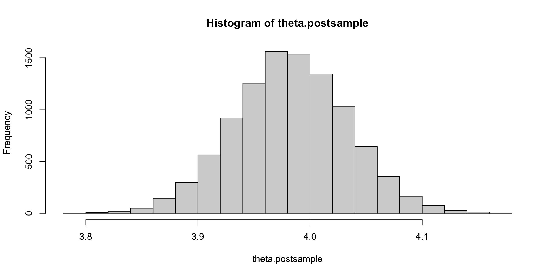
(b). Given the data on the previous slide, use Monte Carlo simulation to plot \(p(\theta | y_1, \ldots, y_n)\). Additionally, report \(E[\theta | y_1,\ldots y_n]\) together with a 95% posterior confidence interval.

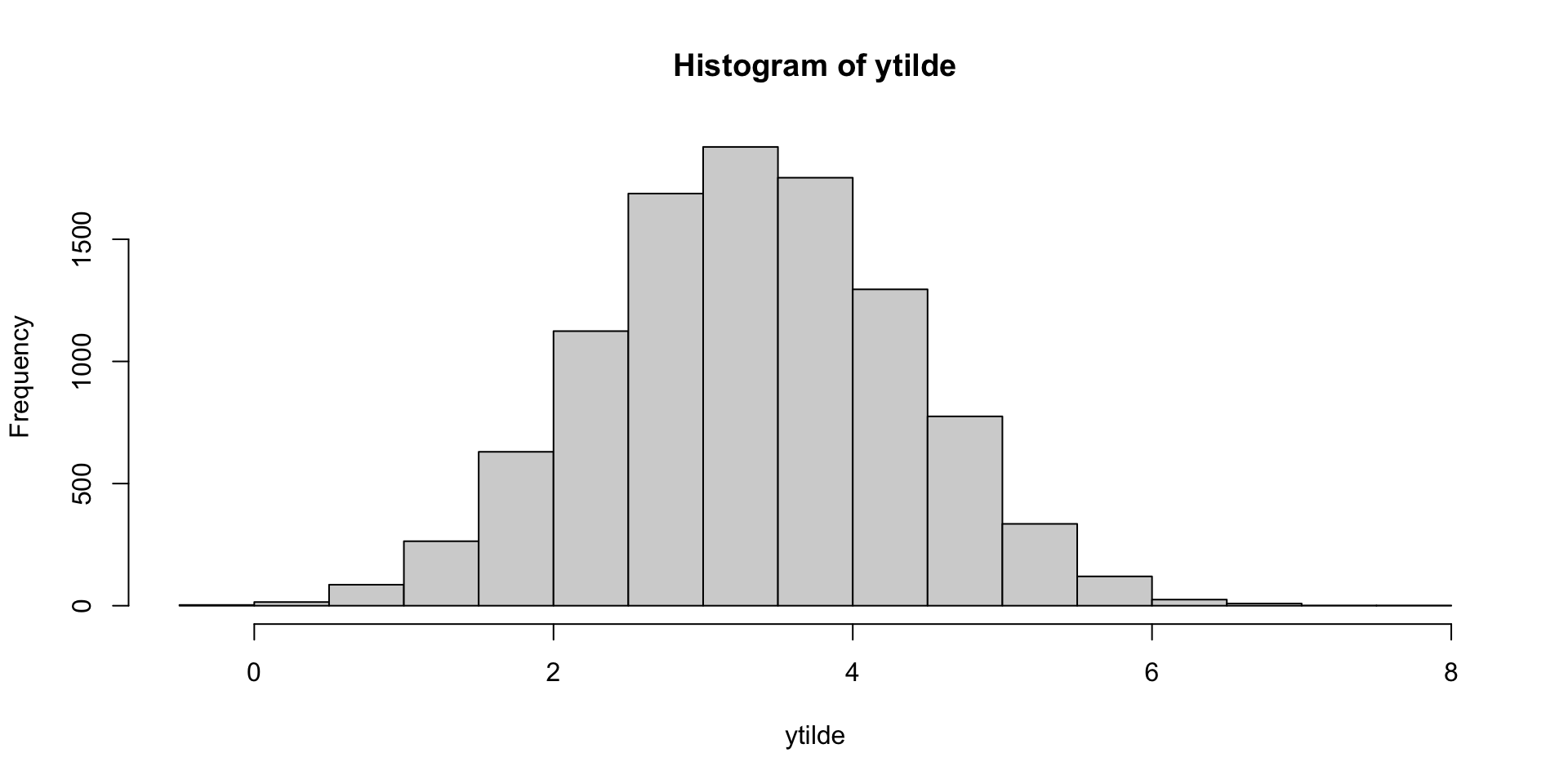
(c). If you caught a new fish with weight 4kg, what would you predict the mercury content to be? In other words, let x = 4 and compute \(E[\tilde{y}|y_1,\ldots, y_n, x = 4]\). Additionally, plot the the posterior predictive density \(p(\tilde{y} | y_1, \ldots y_n, x = 4)\).

(d). Critique your model. Hint: compare to the models below:

lm(mercury ~ weight, data = bass)
lm(mercury ~ 0 + weight, data = bass)

Solution (a)

a

\[ \theta | y_1, \ldots y_n \sim N(\mu_n, \tau_n^2) \]

where

\[ \begin{aligned} \mu_n &= \frac{\kappa_0 \mu_0 + \sum y_i x_i}{\kappa_0 + \sum x_i^2}\\ \tau_n^2 &= \frac{1}{\kappa_0 + \sum x_i^2} \end{aligned} \]

Solution (b)

b

• demo
• demo plot
• solution code
• solution plot
• summary

Demo with simulated data to make sure code works:

# simulated data
set.seed(123)
true.theta = 4
true.sigma = 1
N = 10
x = seq(from = 1, to = 10, length = N)
y = rnorm(N, true.theta * x, true.sigma)

# prior parameters
k0 = 1
mu0 = 0

sumYX = sum(y * x)
d = (k0 + sum(x^2))
mun = ((k0 * mu0) + sumYX) / d
tn = sqrt(1 / d)

theta.postsample = rnorm(10000, mun, tn)
hist(theta.postsample)

x = bass$weight
y = bass$mercury

# prior parameters
k0 = 1
mu0 = 0

sumYX = sum(y * x)
d = (k0 + sum(x^2))
mun = ((k0 * mu0) + sumYX) / d
tn = sqrt(1 / d)

theta.postsample = rnorm(10000, mun, tn)
hist(theta.postsample)

mean(theta.postsample)

[1] 0.8314533

quantile(theta.postsample, c(0.025, 0.975))

     2.5%     97.5% 
0.7284780 0.9356104 

Solution (c)

# use posterior samples of theta and x = 4 to simulate ytilde

ytilde = rnorm(10000, theta.postsample * 4, 1)
hist(ytilde)

mean(ytilde)

[1] 3.319342

This matches intuition (law of total expectation gives the closed form solution: 4 * 0.838 = 3.352).

Solution (d)

We have no intercept term. We are assuming that our regression line goes through the origin. This is a strong assumption. Our model will be most similar to the lm model without an intercept term:

lm(mercury ~ 0 + weight, data = bass)

Call:
lm(formula = mercury ~ 0 + weight, data = bass)

Coefficients:
weight  
0.8343  

However, we’ll get a different estimate of \(\hat{\theta}\) if we include an intercept term,

lm(mercury ~ weight, data = bass)

Call:
lm(formula = mercury ~ weight, data = bass)

Coefficients:
(Intercept)       weight  
     0.6387       0.4818  

Estimators

Exercises

Exercise 1: estimators

Let \(Y_1,\ldots Y_n\) be iid random variables with expectation \(\theta\) and variance \(\sigma^2\).

Show that \(\frac{1}{n} \sum_{i = 1}^n (Y_i -\bar{Y})^2\) is a biased estimator of \(\sigma^2\).

Exercise 2: estimators

\[ \begin{aligned} Y_1, \ldots, Y_n &\sim \text{ i.i.d. binary}(\theta)\\ \theta &\sim \text{beta}(a, b) \end{aligned} \]

• Compute \(\hat{\theta}_{MLE}\)
• Compute \(\hat{\theta}_{B} = E[\theta | y_1,\ldots y_n]\).
• Compare \(MSE(\hat{\theta}_{MLE})\) to \(MSE(\hat{\theta}_{B})\)). Under what conditions is the MSE of \(\hat{\theta}_B\) smaller?

Solutions

Solution 1

Let \(\hat{\sigma}^2 = \frac{1}{n} \sum_{i = 1}^n (Y_i -\bar{Y})^2\).

\[ \begin{aligned} Bias(\hat{\sigma}^2 | \sigma^2 = \sigma_0^2) &= E[\hat{\sigma}^2|\sigma_0^2] - \sigma_0^2\\ &= - \sigma_0^2 + \frac{1}{n} \sum_{i = 1}^n E[(Y_i -\bar{Y})^2|\sigma_0^2]\\ &= - \sigma_0^2 + \frac{1}{n} \sum_{i=1}^n \left[ E[Y_i^2 |\sigma_0^2] - 2E[Y_i \bar{Y}|\sigma_0^2] + E[\bar{Y}^2 | \sigma_0^2] \right] \end{aligned} \]

Recall that for any random variable X, \(Var(X) = E[X^2] - E[X]^2\). Using this fact, we continue our proof above:

\[ \begin{aligned} &= -\sigma_0^2 +(\sigma_0^2 + \theta^2) -2 \frac{1}{n} \sum_{i=1}^n \left[ E~\left(Y_i \frac{1}{n}\sum_j Y_j\right) | \sigma_0^2 \right] + \left(\frac{\sigma_0^2}{n} + \theta^2\right)\\ &= 2\theta^2 + \frac{\sigma_0^2}{n} - \frac{2}{n} \left(n\theta^2 - \sigma_0^2 \right)\\ &= \frac{(n-1)\sigma_0^2}{n} \end{aligned} \]

Solution 2

\[ \begin{aligned} \hat{\theta}_{MLE} &= \bar{Y} = \frac{1}{n}\sum_{i=1}^n Y_i\\ \hat{\theta}_B &= \frac{n\bar{y}+a}{n+a+b} = \end{aligned} \]

\[ \begin{aligned} MSE(\hat{\theta}_{MLE}|\theta) &= \frac{\theta(1-\theta)}{n}\\ MSE(\hat{\theta}_B|\theta) &= \frac{n}{n + a + b}\bar{Y} + \frac{a + b}{n + a + b} \frac{a}{a + b} = w \bar{Y} + (1-w)\frac{a}{a+b}\\ &= w^2Var(\bar{Y} | \theta) + (1-w)^2 \left(\frac{a}{a+b} - \theta\right)^2\\ &= {w^2} \frac{\theta(1-\theta)}{n} + (1-w)^2 \left(\frac{a}{a+b} - \theta\right)^2 \end{aligned} \] For the Bayesian estimator to have smaller MSE than the MLE, we need

\[ \begin{aligned} \left(\frac{a}{a+b} - \theta\right)^2 &\leq \frac{\theta(1 - \theta)}{n} \frac{1 + w}{1 - w}\\ &\leq \frac{\theta(1 - \theta) (2n + a + b)}{n(a+b)} \end{aligned} \]

In words, if our prior guess \(a / (a+b)\) is “close enough” to \(\theta\), where “close enough” is defined by the inequality above and is proportional to the variance of the estimator, then the MSE of the Bayesian estimator is smaller.