Mixture densities
STA602 at Duke University
Definition
What is a mixture density?
A mixture density (sometimes called an “admixture” density) is a convex combination (i.e. weighted sum, with non-negative weights that sum to 1) of other density functions.
In other words…
\[ f(x) = \sum_{i=1}^nw_i p_i(x), \]
where \(p_i(x)\) is a pdf and \(w_i > 0\) for all \(i\) and \(\sum w_i = 1\). We say: \(f(x)\) is a (finite) mixture density.
Mixture densities are often used to model distinct sub-populations within a population. This allows us to create flexible prior distributions.
Exercise
Prove that \(f(x)\) is a proper density function, i.e. that \(f(x) \geq 0\) everywhere and \(\int f(x) dx = 1\).
Practice exercises
Exercise 1
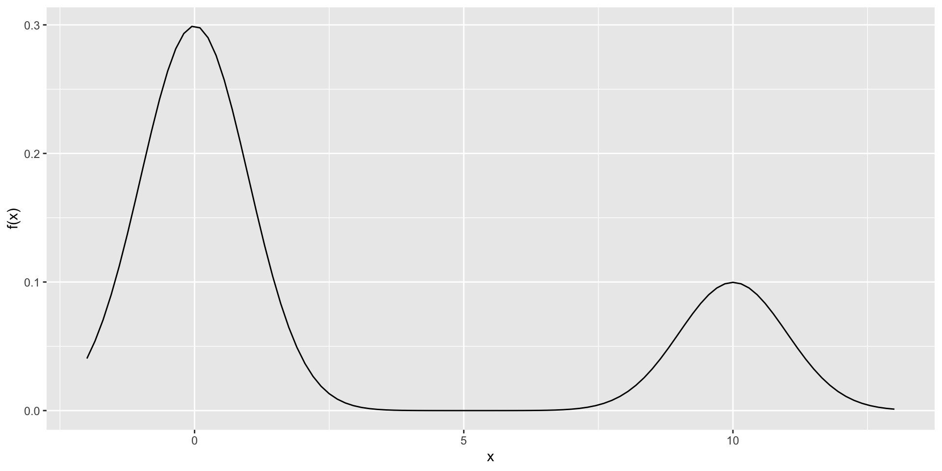
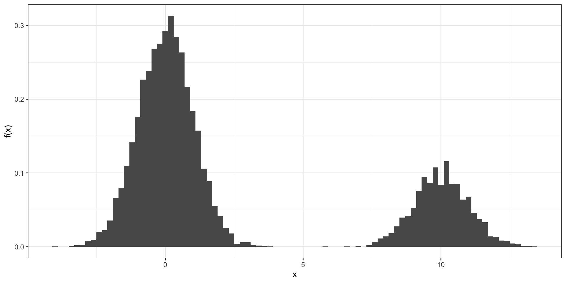
Create and plot a function \(f(x)\) that is a mixture of two densities and approximates the histogram below.
Exercise 2
Suppose an experimental machine in a lab is either fine, or comes from a bad batch of machines that are to be recalled by the manufacturer. Scientists in the lab want to estimate the failure rate of their machine and decide whether or not to return it. They encode their prior uncertainty about the failure rate \(\theta\) with the following density:
\[ p(\theta) = \frac{1}{4} \frac{\Gamma(10)}{\Gamma(2)\Gamma(8)}\left[ 3 \theta (1 - \theta)^7 + \theta^7(1- \theta) \right] \]
(a). Make a plot of this prior density and explain why it makes sense for the scientists. Based on the prior density, which do the scientists think is more likely - that their machine is fine, or bad?
(b). The scientists run the machine \(n\) times. Let \(y_i\) be one if the machine fails on the \(i\)th run, and zero otherwise. Write out the posterior distribution of \(\theta\) given \(y_1, \ldots, y_n\) (up to a proportionality constant) and simplify as much as possible.
(c). The posterior is a mixture (weighted average) of two distributions that you know. Identify these two distributions, including their parameters.
Solutions
Solution 1
The plot looks like a mixture of normals. The first centered on 0 and the second on 10. More weight is given to the first density.
Solution 2
In lab.