MCMC & confidence bands

STA602 at Duke University

Exercises

Setup

Consider the following data generative model and priors:

\[ \begin{aligned} Y_i | \beta_0, \beta_1, x_i &\sim N(\beta_0 + \beta_1x_i, \sigma^2)\\ \beta_0, \beta_1 &\sim \text{ iid } N(0, 2)\\ \sigma^2 &\sim \text{inverse-gamma}(2, 3) \end{aligned} \]

Tip: load library(invgamma) to use the dinvgamma function.

library(tidyverse)
library(invgamma)

# load the data
YX = readr::read_csv("https://sta602-sp25.github.io/data/simulatedXY.csv")
y = YX$y
x = YX$x

Code

Below is code to sample from

\[ p(\beta_1, \beta_2, \sigma^2 | y_1, \ldots, y_n, x_1, \ldots, x_n) \].

set.seed(360)
logLikelihood = function(beta0, beta1, sigma2) {
  mu = beta0 + (beta1 * x)
  sum(dnorm(y, mu, sqrt(sigma2), log = TRUE))
}

logPrior = function(beta0, beta1, sigma2) {
  dnorm(beta0, 0, sqrt(2), log = TRUE) + 
    dnorm(beta1, 0, sqrt(2), log = TRUE) +
    dinvgamma(sigma2, 2, 3, log = TRUE)
}

logPosterior = function(beta0, beta1, sigma2) {
  logLikelihood(beta0, beta1, sigma2) + logPrior(beta0, beta1, sigma2)
}


BETA0 = NULL
BETA1 = NULL
SIGMA2 = NULL

accept1 = 0
accept2 = 0
accept3 = 0

S = 500

beta0_s = 0.1
beta1_s = 10
sigma2_s = 1
for (s in 1:S) {
  
  ## propose and update beta0
  beta0_proposal = rnorm(1, mean = beta0_s, .5)
   log.r = logPosterior(beta0_proposal, beta1_s, sigma2_s) - 
     logPosterior(beta0_s, beta1_s, sigma2_s)
   
   if(log(runif(1)) < log.r)  {
    beta0_s = beta0_proposal
    accept1 = accept1 + 1 
   }
   
   BETA0 = c(BETA0, beta0_s)
   
   ## propose and update beta1
    beta1_proposal = rnorm(1, mean = beta1_s, .5)
   log.r = logPosterior(beta0_s, beta1_proposal, sigma2_s) - 
     logPosterior(beta0_s, beta1_s, sigma2_s)
   
   if(log(runif(1)) < log.r)  {
    beta1_s = beta1_proposal
    accept2 = accept2 + 1 
   }
   
   BETA1 = c(BETA1, beta1_s)
   
   ## propose and update sigma2
   ### note: sigma2 is positive only, we want to only propose positive values
   sigma2_proposal = 1 / rgamma(1, shape = 1, sigma2_s)
   log.r = logPosterior(beta0_s, beta1_s, sigma2_proposal) - 
     logPosterior(beta0_s, beta1_s, sigma2_s) - 
     dinvgamma(sigma2_proposal, 1, sigma2_s, log = TRUE) +
     dinvgamma(sigma2_s, 1, sigma2_proposal, log = TRUE) 
   
   if(log(runif(1)) < log.r)  {
    sigma2_s = sigma2_proposal
    accept3 = accept3 + 1 
   }
   
   SIGMA2 = c(SIGMA2, sigma2_s)
   
}

Exercise 1

Is a Metropolis or Metropolis-Hastings algorithm used to sample \(\sigma^2\)? Hint: What is the proposal distribution used to sample \(\sigma^2\)? Is it symmetric? Can you show that it is or is not symmetric in R?
Create a trace plot for each parameter. How many iterations does it take for \(\beta_1\) to converge to the posterior? What is going on with the \(\sigma^2\) trace plot?
Report the effective sample size of each parameter, \(\beta_0\), \(\beta_1\), and \(\sigma^2\). Hint: load the coda package and check the lecture notes.

Exercise 2

Go back and increase the length of the chain, \(S\), until you obtain approximately 200 ESS for each parameter. Re-examine your plots and discuss.
Report the posterior median and a 90% confidence interval for each unknown. Why is the median a better summary than the mean for \(\sigma^2\)?

Exercise 3

Plot the posterior mean \(\theta(x)\) vs \(x\) where \(\theta(x) \equiv \beta_0 + \beta_1 x\).
Additionally, plot a 95% confidence band for \(\theta(x)\) vs \(x\) and interpret your plot.

Solutions

A Metropolis-Hastings algorithm. inverse-gamma proposal is asymmetric.

Showing with R code:

sigma2_proposal = 1.5
sigma2_s = 1
dinvgamma(sigma2_proposal, 1, sigma2_s) == 
  dinvgamma(sigma2_s, 1, sigma2_proposal)

[1] FALSE

\(\beta_1\) converges to the target after about 50 iterations.
Some samples from inv-gamma are huge, the huge variance results in a flatter likelihood and still get accepted.

library(patchwork)
parameterDF = data.frame(BETA0, BETA1, SIGMA2)
n = nrow(parameterDF)

p0 = parameterDF %>%
  ggplot(aes(x = 1:n)) +
  geom_line(aes(y = BETA0)) +
  theme_bw() +
  labs(x = "iteration", y = "beta0")

p1 = parameterDF %>%
  ggplot(aes(x = 1:n)) +
  geom_line(aes(y = BETA1)) +
  theme_bw() +
  labs(x = "iteration", y = "beta1")

p2 = parameterDF %>%
  ggplot(aes(x = 1:n)) +
  geom_line(aes(y = SIGMA2)) +
  theme_bw() +
  labs(x = "iteration", y = "sigma2")

p0 + p1 + p2

library(coda) 

parameterDF = data.frame(BETA0, BETA1, SIGMA2)
apply(parameterDF, 2, effectiveSize)

   BETA0    BETA1   SIGMA2 
19.47526 11.66309 26.31348

set.seed(360)
logLikelihood = function(beta0, beta1, sigma2) {
  mu = beta0 + (beta1 * x)
  sum(dnorm(y, mu, sqrt(sigma2), log = TRUE))
}

logPrior = function(beta0, beta1, sigma2) {
  dnorm(beta0, 0, sqrt(2), log = TRUE) + 
    dnorm(beta1, 0, sqrt(2), log = TRUE) +
    dinvgamma(sigma2, 2, 3, log = TRUE)
}

logPosterior = function(beta0, beta1, sigma2) {
  logLikelihood(beta0, beta1, sigma2) + logPrior(beta0, beta1, sigma2)
}


BETA0 = NULL
BETA1 = NULL
SIGMA2 = NULL

accept1 = 0
accept2 = 0
accept3 = 0

S = 10000

beta0_s = 0.1
beta1_s = 10
sigma2_s = 1
for (s in 1:S) {
  
  ## propose and update beta0
  beta0_proposal = rnorm(1, mean = beta0_s, .5)
   log.r = logPosterior(beta0_proposal, beta1_s, sigma2_s) - 
     logPosterior(beta0_s, beta1_s, sigma2_s)
   
   if(log(runif(1)) < log.r)  {
    beta0_s = beta0_proposal
    accept1 = accept1 + 1 
   }
   
   BETA0 = c(BETA0, beta0_s)
   
   ## propose and update beta1
    beta1_proposal = rnorm(1, mean = beta1_s, .5)
   log.r = logPosterior(beta0_s, beta1_proposal, sigma2_s) - 
     logPosterior(beta0_s, beta1_s, sigma2_s)
   
   if(log(runif(1)) < log.r)  {
    beta1_s = beta1_proposal
    accept2 = accept2 + 1 
   }
   
   BETA1 = c(BETA1, beta1_s)
   
   ## propose and update sigma2
   ### note: sigma2 is positive only, we want to only propose positive values
   sigma2_proposal = 1 / rgamma(1, shape = 1, sigma2_s)
   log.r = logPosterior(beta0_s, beta1_s, sigma2_proposal) - 
     logPosterior(beta0_s, beta1_s, sigma2_s) - 
     dinvgamma(sigma2_proposal, 1, sigma2_s, log = TRUE) + 
     dinvgamma(sigma2_s, 1, sigma2_proposal, log = TRUE) 
   
   if(log(runif(1)) < log.r)  {
    sigma2_s = sigma2_proposal
    accept3 = accept3 + 1 
   }
   
   SIGMA2 = c(SIGMA2, sigma2_s)
   
}

parameterDF = data.frame(BETA0, BETA1, SIGMA2)
apply(parameterDF, 2, effectiveSize)

   BETA0    BETA1   SIGMA2 
939.9746 377.1986 580.0570

	post. median	CI
beta0	0.6	(-0.4, 1.5)
beta1	2	(1.9, 2.1)
sigma2	11.6	(7.1, 20.6)

Solution 3

plot
code

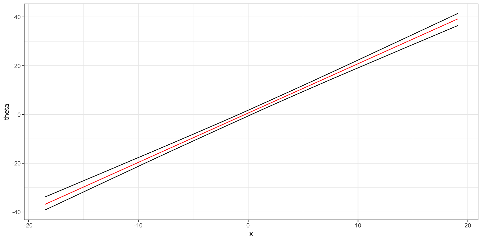
The red line shows our posterior expectation of \(\theta(x)\) for each \(x\). The black bands show our 95% confidence interval \(\theta(x)\).

get_theta_CI = function(X) {
     f = BETA0 + (BETA1 * X)
     return(quantile(f, c(0.025, 0.975)))
}

get_theta_mean = function(X) {
  f = BETA0 + (BETA1 * X)
  return(mean(f))
}

xlo = min(x)
xhi = max(x)
xVal = seq(xlo, xhi, by = 0.01)
lower = NULL
upper = NULL
M = NULL
   
for (i in seq_along(xVal)) {
  theta_CI = get_theta_CI(xVal[i])
  lower = c(lower, theta_CI[[1]])
  upper = c(upper, theta_CI[[2]])
  M = c(M, get_theta_mean(xVal[i]))
}

df = data.frame(xVal, lower, upper, M)
df %>%
  ggplot(aes(x = xVal)) +
  geom_line(aes(y = lower)) +
  geom_line(aes(y = upper)) +
  geom_line(aes(y = M), col = "red") +
  theme_bw() +
  labs(y = "theta",
       x = "x")