Water on Mars

Author

Dr. Alexander Fisher

load libraries

library(truncnorm)
library(tidyverse)
library(coda)

Bayesian inverse problems

Idea: writing the likelihood is difficult or impossible in closed form.

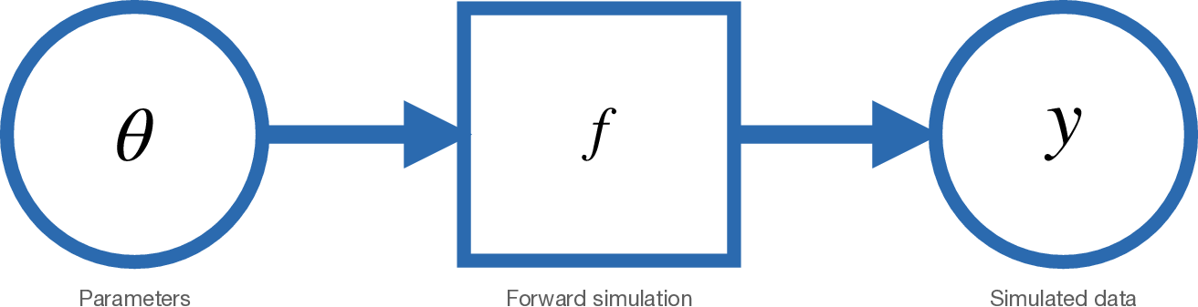
As usual, we wish to estimate some parameter vector \(\theta\). However, \(\theta\) relates to our observations \(y\) via some function \(y = f(\theta)\). The catch is, we cannot write \(f(\theta)\) directly, nor compute it exactly. Most often, all we can do is simulate from \(f(\theta)\).

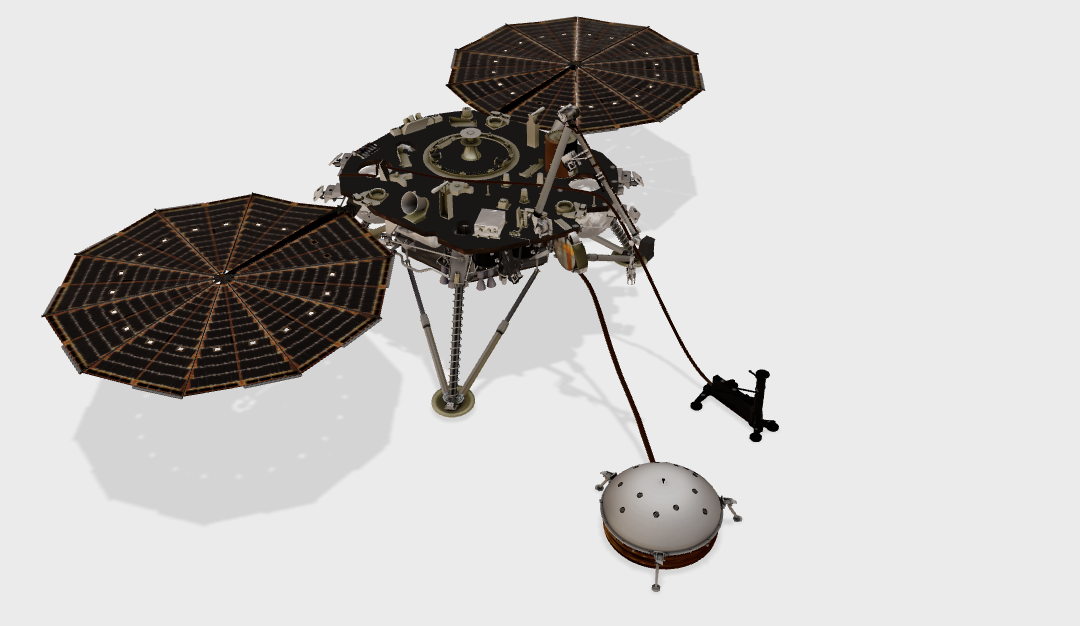
Example: Liquid water in the Martian mid-crust ¹

InSight. Photo credit: NASA. Image retrieved from https://science.nasa.gov/mission/insight/

The Interior Exploration using Seismic Investigations, Geodesy and Heat Transport (InSight) mission from NASA sent a robotic lander to Mars on May 5, 2018. The goal of the mission, which ended December 2022, was to study the crust, mantle and core of Mars.

Data

Watch the video here to see the data that InSight collects from earthquakes on Mars.

seismic_data = data.frame(y = c(4.1, 2.5, 2589),
                          sd = c(0.2, 0.3, 157))

Parameter Table

Here our parameter vector \(\theta = (\alpha, \phi, \gamma_w, \kappa_m, \mu_m, \rho_m)\). These parameters describe the medium through which the earthquake waves propagate.

Symbol in paper	Code	Definition
\(\alpha\)	`theta[1]`	Pore shape aspect ratio
\(\phi\)	`theta[2]`	Porosity
\(\gamma_w\)	`theta[3]`	Water saturation (%)
\(\kappa_m\)	`theta[4]`	Mineral bulk modulus (GPa)
\(\mu_m\)	`theta[5]`	Mineral shear modulus (GPa)
\(\rho_m\)	`theta[6]`	Mineral density (kg/m\(^3\))

Berryman self-consistent rock physics model

The function \(f(\theta)\) that forward simulates data given our set of parameters is myBerry in the code below. This function serves as a wrapper to the berry_scm function, also defined below. Functions are translated into R from original MATLAB code by Wright, Morzfeld and Manga from the paper and publicly available on GitHub. ²

Show Berryman functions

berry_scm <- function(k, mu, asp, x, ro1, P_water) {
  # BERRYSCM - Effective elastic moduli for multi-component composite
  # using Berryman's Self-Consistent (Coherent Potential Approximation) method.
  # 
  # Arguments:
  # k: Bulk moduli of the N constituent phases (numeric vector)
  # mu: Shear moduli of the N constituent phases (numeric vector)
  # asp: Aspect ratio for the inclusions of the N phases (numeric vector)
  # x: Fraction of each phase. Solid, then fluid phase (numeric vector)
  # ro1: Density of the original rock (numeric scalar)
  # P_water: Proportion of water (numeric scalar)
  #
  # Returns:
  # kbr: Effective bulk modulus (numeric scalar)
  # mubr: Effective shear modulus (numeric scalar)
  # vp: P-wave velocity (numeric scalar)
  # vs: S-wave velocity (numeric scalar)
  # ro2: Final rock density after fluid substitution (numeric scalar)
  # k2: Rock bulk modulus after fluid substitution (numeric scalar)
  
  # Ensure inputs are column vectors (equivalent to MATLAB's k(:), mu(:), etc.)
  k <- as.vector(k)
  mu <- as.vector(mu)
  asp <- as.vector(asp)
  x <- as.vector(x)
  
  # Modify aspect ratios of inclusions that are equal to 1
  asp[asp == 1] <- 0.99
  
  # Initialize variables
  theta <- numeric(length(asp))
  fn <- numeric(length(asp))
  
  # Compute theta and fn for oblate and prolate spheroids
  obdx <- which(asp < 1)
  prdx <- which(asp > 1)
  
  theta[obdx] <- (asp[obdx] / ((1 - asp[obdx]^2)^(3/2))) * (acos(asp[obdx]) - asp[obdx] * sqrt(1 - asp[obdx]^2))
  fn[obdx] <- (asp[obdx]^2 / (1 - asp[obdx]^2)) * (3 * theta[obdx] - 2)
  
  theta[prdx] <- (asp[prdx] / ((asp[prdx]^2 - 1)^(3/2))) * (asp[prdx] * sqrt(asp[prdx]^2 - 1) - acosh(asp[prdx]))
  fn[prdx] <- (asp[prdx]^2 / (asp[prdx]^2 - 1)) * (2 - 3 * theta[prdx])
  
  # Initialize initial bulk and shear moduli
  ksc <- sum(k * x)
  musc <- sum(mu * x)
  
  # Initialize iteration parameters
  knew <- 0
  tol <- 1e-6 * k[1]
  del <- abs(ksc - knew)
  niter <- 0
  
  # Iterative solution for effective moduli
  while (del > abs(tol) && niter < 3000) {
    nusc <- (3 * ksc - 2 * musc) / (2 * (3 * ksc + musc))
    a <- mu / musc - 1
    b <- (1 / 3) * (k / ksc - mu / musc)
    r <- (1 - 2 * nusc) / (2 * (1 - nusc))
    
    f1 <- 1 + a * ((3 / 2) * (fn + theta) - r * ((3 / 2) * fn + (5 / 2) * theta - (4 / 3)))
    f2 <- 1 + a * (1 + (3 / 2) * (fn + theta) - (r / 2) * (3 * fn + 5 * theta)) + b * (3 - 4 * r)
    f2 <- f2 + (a / 2) * (a + 3 * b) * (3 - 4 * r) * (fn + theta - r * (fn - theta + 2 * theta^2))
    f3 <- 1 + a * (1 - (fn + (3 / 2) * theta) + r * (fn + theta))
    f4 <- 1 + (a / 4) * (fn + 3 * theta - r * (fn - theta))
    f5 <- a * (-fn + r * (fn + theta - (4 / 3))) + b * theta * (3 - 4 * r)
    f6 <- 1 + a * (1 + fn - r * (fn + theta)) + b * (1 - theta) * (3 - 4 * r)
    f7 <- 2 + (a / 4) * (3 * fn + 9 * theta - r * (3 * fn + 5 * theta)) + b * theta * (3 - 4 * r)
    f8 <- a * (1 - 2 * r + (fn / 2) * (r - 1) + (theta / 2) * (5 * r - 3)) + b * (1 - theta) * (3 - 4 * r)
    f9 <- a * ((r - 1) * fn - r * theta) + b * theta * (3 - 4 * r)
    
    p <- 3 * f1 / f2
    q <- (2 / f3) + (1 / f4) + ((f4 * f5 + f6 * f7 - f8 * f9) / (f2 * f4))
    
    p <- p / 3
    q <- q / 5
    
    # Update moduli
    knew <- sum(x * k * p) / sum(x * p)
    munew <- sum(x * mu * q) / sum(x * q)
    
    del <- abs(ksc - knew)
    ksc <- knew
    musc <- munew
    niter <- niter + 1
  }
  
  kbr <- ksc
  mubr <- musc
  
  # Density and fluid substitution
  rofl1 <- 0.020    # density of gas
  kfl1 <- 0         # bulk modulus of gas
  ro_water <- 1000   # density of water
  k_water <- 2.2e9  # bulk modulus of water
  P_gas <- 1 - P_water
  rofl2 <- P_gas * rofl1 + P_water * ro_water
  kfl2 <- P_gas * kfl1 + P_water * k_water
  k0 <- k[1]        # bulk modulus of solid mineral phase
  phi <- x[2]       # porosity of rock
  k1 <- kbr         # dry bulk modulus
  
  # Perform fluid substitution using Gassmann equation
  a <- k1 / (k0 - k1) - kfl1 / (phi * (k0 - kfl1)) + kfl2 / (phi * (k0 - kfl2))
  k2 <- k0 * a / (1 + a)   # bulk modulus after fluid substitution
  
  # Compute final density after fluid substitution
  ro2 <- ro1 - phi * rofl1 + phi * rofl2
  
  # Compute seismic velocities after fluid substitution
  mu2 <- mubr
  vp <- sqrt((k2 + (4 / 3) * mu2) / ro2)
  vs <- sqrt(mu2 / ro2)
  
  return(list(kbr = kbr, mubr = mubr, vp = vp, vs = vs, ro2 = ro2, k2 = k2))
}

myBerry <- function(theta, H = 3) {
  # Extract parameters from theta
  asp <- c(1, theta[1])   # Aspect ratio
  x_phi <- theta[2]       # Proportion of fluid (phi)
  rock_vol <- 1 - theta[2] # Volume of solid phase (rock)
  x <- c(rock_vol, x_phi)  # Fraction of phases
  rock_density <- theta[6] * rock_vol  # Density of solid phase (basalt)
  gas_density <- 0.020 * x_phi         # Density of fluid phase (gas)
  rhob1 <- rock_density + gas_density  # Bulk density
  
  # Percentage of water in pore space
  P_water <- theta[3]
  
  # Bulk and shear moduli (scaled by 1e9 as per MATLAB code)
  k <- c(theta[4] * 1e9, 0)  # Bulk modulus (first element)
  mu <- c(theta[5] * 1e9, 0) # Shear modulus (first element)
  
  # Call berryscm function (ensure berryscm function is defined in your R environment)
  result <- berry_scm(k, mu, asp, x, rhob1, P_water)
  
  # Return the required output from berryscm
  return(result)
}

Likelihood and prior

Exercise

Why does a normal likelihood make sense?

What priors are chosen for each unknown?

Inference

Code

set.seed(360)
dtruncnormL = function(x, a, b, mean, sd) {
  log(dtruncnorm(x, a=a, b=b, mean = mean, sd = sd))
}

rcnorm<-function(n, mean=0, sd=1, a=-Inf, b=Inf){
  u = runif(n, pnorm((a - mean) / sd), pnorm((b - mean) / sd))
  mean + (sd * qnorm(u))
}

logPosterior = function(theta) {
  result = myBerry(theta)
  y = c(result$vp / 1000, result$vs / 1000, result$ro2)
  if(result$vp < result$vs) {
    return(-Inf)
  }
  else{
  return(
    sum(dnorm(y, mean = seismic_data$y, sd = seismic_data$sd,
            log = TRUE))
  )
  }
}

# THETA[1] = alpha
# THETA[2] = porosity
# THETA[3] = saturation
# THETA[4] = kappa_m
# THETA[5] = mu_m
# THETA[6] = rho_m

# starting point
alpha = 0.5
porosity = 0.25 #runif(1, 0.05, 0.50)
saturation = 0.05 #0 to 1
kappa_m = 78
mu_m = 33
rhom = 3000
theta = c(alpha, porosity, saturation, kappa_m, mu_m, rhom)

# prior
## indicator that parameters are in proper ranges * constant * indicator that Vp > Vs

# MCMC 
S = 50000
accept = rep(0, length(theta))

THETA = NULL
for(i in 1:S) {
  thetaStar = theta 
  thetaStar[1] = rcnorm(1, mean = theta[1], sd = .05,
                        a = 0.03, b = 0.99)
   log.r = logPosterior(thetaStar) + 
     dtruncnormL(theta[1], 
                a=0.03, b=0.99, 
                mean = thetaStar[1], sd = .05) - 
     logPosterior(theta) - 
     dtruncnormL(thetaStar[1], 
                a=0.03, b=0.99, 
                mean = theta[1], sd = .05)
   
   if(log(runif(1)) < log.r)  {
    theta = thetaStar
    accept[1] = accept[1] + 1 
   }
  
  thetaStar = theta
  thetaStar[2] = rcnorm(1, mean = theta[2], sd = .05,
                        a = 0.05, b = 0.5)
  log.r = logPosterior(thetaStar) +
    dtruncnormL(thetaStar[2], 
                a=0.05, b=0.5, 
                mean = theta[2], sd = .05) - 
     logPosterior(theta) - 
      dtruncnormL(thetaStar[2], 
                a=0.05, b=0.5, 
                mean = theta[2], sd = .05)
   
   if(log(runif(1)) < log.r)  {
    theta = thetaStar
    accept[2] = accept[2] + 1 
   }
  
  thetaStar = theta
  thetaStar[3] = rcnorm(1, mean = theta[3], sd = 0.05,
                        a = 0, b = 1)
  
  log.r = logPosterior(thetaStar) +
    dtruncnormL(thetaStar[3], 
                a=0, b=1, 
                mean = theta[3], sd = 0.05) - 
     logPosterior(theta) - 
    dtruncnormL(thetaStar[3], 
                a=0, b=1, 
                mean = theta[3], sd = 0.05)
   
   if(log(runif(1)) < log.r)  {
    theta = thetaStar
    accept[3] = accept[3] + 1 
   }
  
  thetaStar = theta
  thetaStar[4] = rcnorm(1, mean = theta[4], sd = .5,
                        a = 76.5, b = 80)
  
  log.r = logPosterior(thetaStar) +
    dtruncnormL(thetaStar[4], 
                a=76.5, b=80, 
                mean = theta[4], sd = .5) - 
     logPosterior(theta) -
    dtruncnormL(thetaStar[4], 
                a=76.5, b=80, 
                mean = theta[4], sd = .5)
   
   if(log(runif(1)) < log.r)  {
    theta = thetaStar
    accept[4] = accept[4] + 1 
   }
  
  thetaStar = theta
  thetaStar[5] = rcnorm(1, mean = theta[5], sd = 1,
                        a = 25.6, b = 40)
  
  log.r = logPosterior(thetaStar) +
    dtruncnormL(thetaStar[5], 
                a=25.6, b=40, 
                mean = theta[5], sd = 1) - 
     logPosterior(theta) -
    dtruncnormL(thetaStar[5], 
                a=25.6, b=40, 
                mean = theta[5], sd = 1)
   
   if(log(runif(1)) < log.r)  {
    theta = thetaStar
    accept[5] = accept[5] + 1 
   }
  
  thetaStar = theta
  thetaStar[6] = rcnorm(1, mean = theta[6], sd = 20,
                        a = 2689, b = 2900)
  
   log.r = logPosterior(thetaStar) +
    dtruncnormL(thetaStar[6], 
                a=2689, b=2900, 
                mean = theta[6], sd = 20) - 
     logPosterior(theta) -
    dtruncnormL(thetaStar[6], 
                a=2689, b=2900, 
                mean = theta[6], sd = 20)
   
   if(log(runif(1)) < log.r)  {
    theta = thetaStar
    accept[6] = accept[6] + 1 
   }
  
   THETA = rbind(THETA, theta)
}

Code

N = nrow(THETA)
THETA = THETA %>%
  mutate(iteration = seq(1,N))

THETA %>%
  filter(iteration > 30000) %>%
  pivot_longer(cols = 1:6) %>%
  ggplot(aes(x = iteration, y = value)) +
  geom_line() +
  facet_wrap(~ name, scales = "free_y")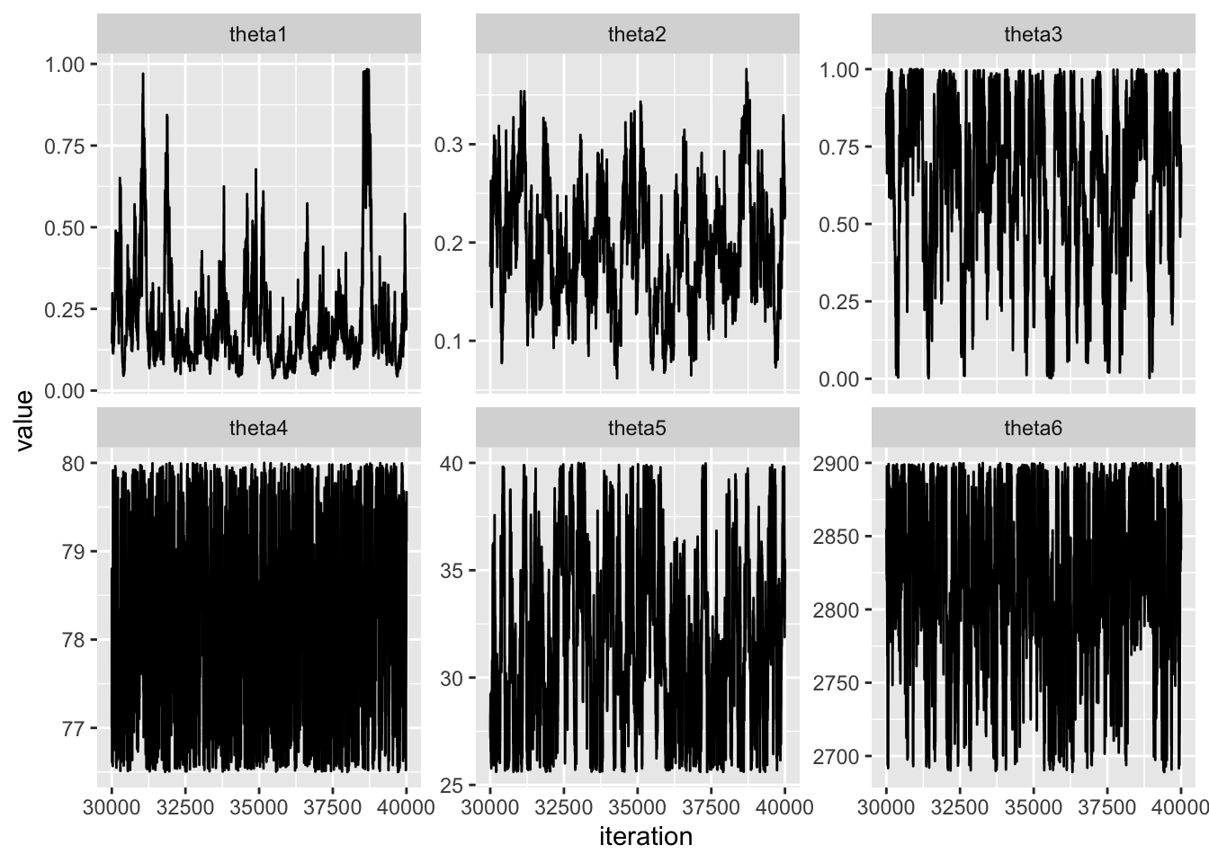

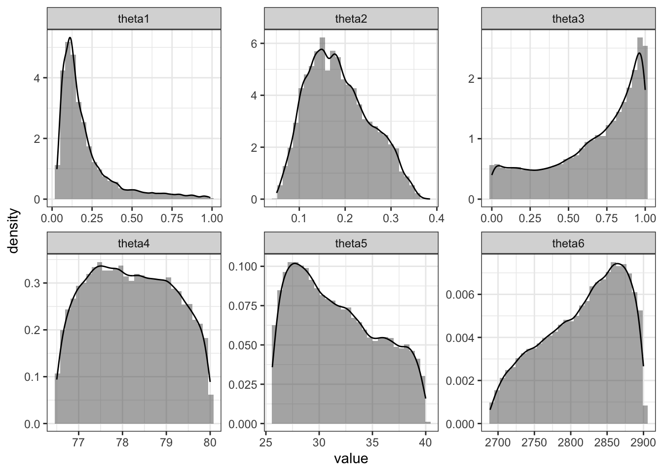
Code

THETA %>%
  filter(iteration > 20000) %>%
  pivot_longer(cols = 1:6) %>%
  ggplot(aes(x = value)) +
  geom_histogram(aes(y = ..density..), alpha = 0.5) +
  geom_density() +
  facet_wrap(~ name, scales = "free") +
  theme_bw()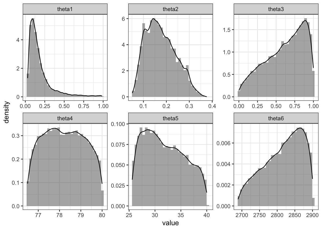

Code

library(knitr)
# posterior means of parameters
posteriorMeans = 
  THETA %>%
  select(-iteration) %>%
  colMeans()

posteriorMeans %>% 
  kable(col.names = c("parameter", "posteriorMean"))

parameter	posteriorMean
theta1	0.2083255
theta2	0.1831104
theta3	0.5988736
theta4	78.2017496
theta5	31.7572690
theta6	2816.4036103

Code

# generating data from posterior means 
result = myBerry(posteriorMeans)
dataFromPostMean = c(result$vp / 1000, result$vs / 1000, result$ro2)
rbind(dataFromPostMean, seismic_data$y) %>%
  kable(col.names = c("Vp", "Vs", "Rho"), digits = 3)

	Vp	Vs	Rho
dataFromPostMean	4.603	2.596	2410.352
	4.100	2.500	2589.000

Discussion

Prior sensitivity

Exercise

Discuss with a neighbor: do you think the results are sensitive to the choice of prior?

Alternate prior
Marginal posteriors

\(beta(1/2, 1/2)\) prior on water saturation.

logPosterior = function(theta) {
  result = myBerry(theta)
  y = c(result$vp / 1000, result$vs / 1000, result$ro2)
  if(result$vp < result$vs) {
    return(-Inf)
  }
  else{
  return(
    sum(dnorm(y, mean = seismic_data$y, sd = seismic_data$sd,
            log = TRUE)) + 
      dbeta(theta[3], .5, .5, log = TRUE)
  )
  }
}

Model selection

Let \(M_1\) be the hypothesis that there is water present under the surface of Mars and let \(M_0\) be the hypothesis that there is not. Really, we want to select between these two hypotheses.

To do this, consider the ratio of posterior probabilities

\[ \begin{aligned} \underbrace{\frac{Pr(M_1 | data)}{Pr(M_0 |data)}}_{\text{posterior odds}} = \underbrace{\frac{p({data} | M_1)}{p(data | M_0}}_{\text{Bayes factor}} \underbrace{\frac{p(M_1)}{p(M_0)}}_{\text{prior odds}} \end{aligned} \]

The Bayes factor tells us how the data supports one hypothesis over another. Notice that we cannot compute the Bayes factor directly. We must expand,

\[ \begin{aligned} p(data | M_i) &= \int p(data, \theta | M_i) d\theta\\ &= \int p(data | \theta) p(\theta | M_i) d \theta \end{aligned} \]

Important

Notice that the Bayes factor does depend on the prior \(p(\theta | M_i)\).

Footnotes

Wright, V., Morzfeld, M., & Manga, M. (2024). Liquid water in the Martian mid-crust. Proceedings of the National Academy of Sciences, 121(35), e2409983121.↩︎
https://github.com/mattimorzfeld/WMM24 ↩︎

Bayesian inverse problems

Example: Liquid water in the Martian mid-crust 1

Data

Parameter Table

Berryman self-consistent rock physics model

Likelihood and prior

Inference

Discussion

Prior sensitivity

Model selection

Footnotes

Example: Liquid water in the Martian mid-crust ¹