view packages used in these notes
# load packages
library(tidyverse)
library(coda)# load packages
library(tidyverse)
library(coda)Each year, students across North Carolina take an identical standardized test. In our sample, we observe scores from students at \(m\) different schools. At the \(j\)th school, \(n_j\) students take the exam and \(j \in \{1, \ldots m\}\). The exam is designed to give an average score of 50 on a 0 to 100 scale.
# load data
mathScores = read_csv("https://sta360-fa24.github.io/data/mathScores.csv")school: which school the math score came frommathscore: score from 0 to 100 of an individual studentRows: 1,993
Columns: 2
$ school <dbl> 1, 1, 1, 1, 1, 1, 1, 1, 1, 1, 1, 1, 1, 1, 1, 1, 1, 1, 1, 1, …
$ mathscore <dbl> 52.11, 57.65, 66.44, 44.68, 40.57, 35.04, 50.71, 66.17, 39.4…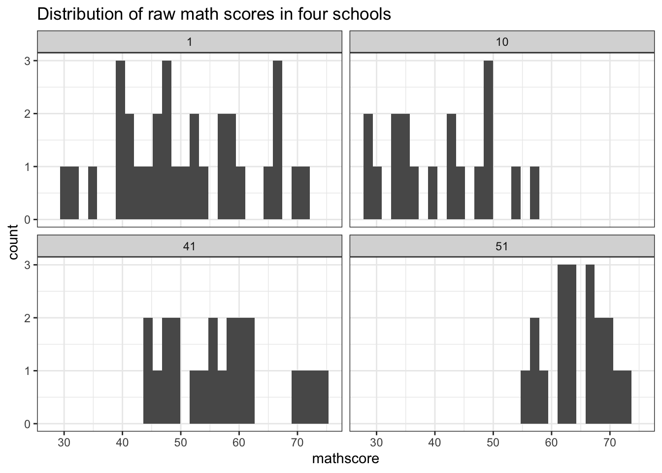
Y.school.mathscore <- as.matrix(mathScores)
#### Put data into list form.
Y <- list()
J <- max(Y.school.mathscore[, 1])
n <- ybar <- ymed <- s2 <- rep(0, J)
for (j in 1:J) {
  Y[[j]] <- Y.school.mathscore[Y.school.mathscore[, 1] == j, 2]
}Suppose students scores at school \(j\) are exchangeable for all \(n_j\). By de Finetti’s theorem, this means
\[ \{y_{1,j}, \ldots y_{n_j,j} | \phi_j \} \sim \text{ i.i.d. } p(y|\phi_j). \] That is, the student’s scores at school \(j\) are conditionally i.i.d. given some school specific parameters \(\phi_j\). This describes our within-group sampling variability.
Now suppose that all the schools we sampled are similar in some way. Maybe they belong to some larger population of schools across the country i.e. schools in North Carolina are somewhat distinct from schools in South Carolina. We might imagine that the school-specific parameters themselves are exchangeable for all \(m\). By de Finetti’s theorem, this means
\[ \{\phi_1, \ldots \phi_m\} \sim \text{ i.i.d. } p(\phi|\psi). \]
In words, school-specific parameters are conditionally i.i.d. given some population specific parameters \(\psi\). This describes our between-group sampling variability.
Finally, if our hierarchy stops there, then to complete model specification, we may describe our prior beliefs about \(\psi\) according to some prior density \(p(\psi)\).
Imagine variability among scores is the same across all schools, but there does exist heterogeneity in the mean scores of the schools. Write down the mathematical form of a model that describes this using the normal distribution. What are some priors you could pick on relevant parameters to make sure full conditionals are easy to compute for Gibbs sampling? What are the full conditionals?
\[ \begin{aligned} y_j | \theta_j, \sigma^2 &\sim N(\theta_j, \sigma^2)\\ \theta_j | \mu, \tau^2 &\sim N(\mu, \tau^2) \end{aligned} \]
\[ \begin{aligned} 1/\sigma^2 &\sim \text{ gamma}(\nu_0/2, \nu_0 \sigma_0^2/2)\\ 1/\tau^2 &\sim \text{ gamma}(\eta_0/2, \eta_0 \tau_0^2/2)\\ \mu &\sim N(\mu_0, \gamma_0^2) \end{aligned} \]
To facilitate Gibbs sampling, notice
\[ p(\theta_1, \ldots \theta_m, \mu, \tau^2, \sigma^2 | \mathbf{y}_1, \ldots \mathbf{y}_m) \propto p(\mu, \tau^2, \sigma^2) p(\theta_1, \ldots \theta_m | \mu, \tau^2, \sigma^2) \times p(\mathbf{y}_1, \ldots \mathbf{y}_m| \theta_1, \ldots \theta_m, \mu, \tau^2, \sigma^2) \]
It follows that the full conditionals are:
\[ \begin{aligned} p(\mu | \cdot) &\propto p(\mu) \prod_{j = 1}^m p(\theta_j| \mu, \tau^2)\\ p(\tau^2 | \cdot) &\propto p(\tau^2) \prod_{j = 1}^m p(\theta_j| \mu, \tau^2)\\ p(\sigma^2|\cdot) &\propto p(\sigma^2)\prod_{j =1}^m \prod_{i = 1}^{n_j} p(y_{i,j}|\theta_j, \sigma^2)\\ p(\theta_j | \cdot) &\propto p(\theta_j | \mu, \tau^2) \prod_{i = 1}^{n_j} p(y_{i,j}|\theta_j, \sigma^2) \end{aligned} \]
#### MCMC approximation to posterior for the hierarchical normal model

## weakly informative priors
nu0 <- 1; s20 <- 100
eta0 <- 1; t20 <- 100
mu0 <- 50; g20 <- 25

## starting values
m <- length(Y)
n <- sv <- ybar <- rep(NA, m)
for (j in 1:m)
{
  ybar[j] <- mean(Y[[j]])
  sv[j] <- var(Y[[j]])
  n[j] <- length(Y[[j]])
}
theta <- ybar
sigma2 <- mean(sv)
mu <- mean(theta)
tau2 <- var(theta)

## setup MCMC
set.seed(1)
S <- 5000
THETA <- matrix(nrow = S, ncol = m)
MST <- matrix(nrow = S, ncol = 3)
predictiveY = NULL

## MCMC algorithm
for (s in 1:S)
{
  # sample new values of the thetas
  for (j in 1:m)
  {
    vtheta <- 1 / (n[j] / sigma2 + 1 / tau2)
    etheta <- vtheta * (ybar[j] * n[j] / sigma2 + mu / tau2)
    theta[j] <- rnorm(1, etheta, sqrt(vtheta))
  }

  #sample new value of sigma2
  nun <- nu0 + sum(n)
  ss <- nu0 * s20
  for (j in 1:m) {
    ss <- ss + sum((Y[[j]] - theta[j]) ^ 2)
  }
  sigma2 <- 1 / rgamma(1, nun / 2, ss / 2)

  #sample a new value of mu
  vmu <- 1 / (m / tau2 + 1 / g20)
  emu <- vmu * (m * mean(theta) / tau2 + mu0 / g20)
  mu <- rnorm(1, emu, sqrt(vmu))

  # sample a new value of tau2
  etam <- eta0 + m
  ss <- eta0 * t20 + sum((theta - mu) ^ 2)
  tau2 <- 1 / rgamma(1, etam / 2, ss / 2)

  #store results
  THETA[s, ] <- theta
  MST[s, ] <- c(mu, sigma2, tau2)

  # predictive sampling
  y51 = rnorm(1, mean = theta[51], sd = sqrt(sigma2))
  y41 = rnorm(1, mean = theta[41], sd = sqrt(sigma2))
  predictiveY = rbind(predictiveY, c(y51, y41))

}

mcmc1 <- list(THETA = THETA, MST = MST)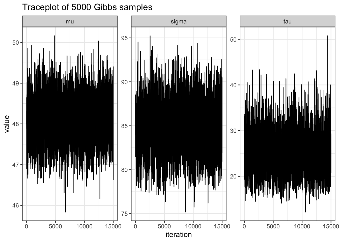
colnames(MST) = c("mu", "sigma2", "tau2")
MST2 = MST %>%
  as.data.frame() %>%
  pivot_longer(cols = 1:3)

MST2 %>%
  ggplot(aes(x = seq(1, nrow(MST2)), y = value)) +
  geom_line() +
  theme_bw() +
  facet_wrap(~ name, scales = "free_y") +
  labs(y = "mu",
       x = "iteration",
title = "Traceplot of 5000 Gibbs samples")effectiveSize(MST) mu sigma tau
3925.336 4461.112 2905.517 par(mfrow=c(1,3))
acf(MST[,1])
acf(MST[,2])
acf(MST[,3]) 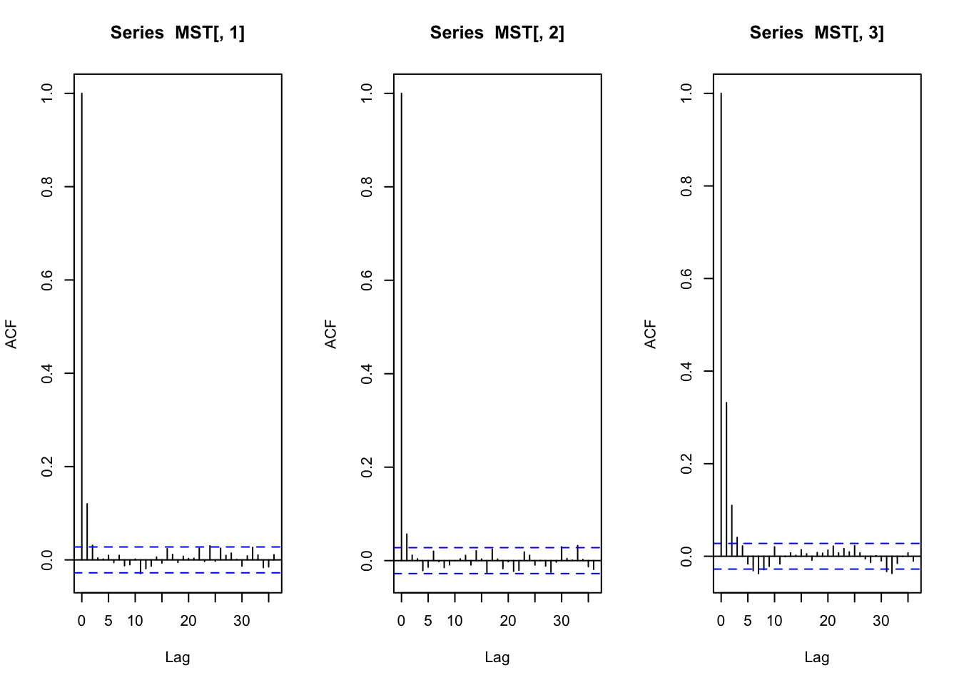
# MC error of mu, sigma2, tau2
MCERR <- apply(MST,2,sd)/sqrt( effectiveSize(MST) )
apply(MST,2,mean)
mu sigma tau
48.12530 84.82892 24.79410 MCERR mu sigma tau
0.008528321 0.041664073 0.082344432 We can do the exact same for the thetas, but the output will be 100 lines, so I suppress output below.
# MC error of thetas
effectiveSize(THETA) -> esTHETA
TMCERR <- apply(THETA,2,sd)/sqrt( effectiveSize(THETA) )
TMCERR# Ordering E[theta | data] and comparing to ybar
posteriorMean = THETA %>%
apply(2, mean)
orderedTable = mathScores %>%
group_by(school) %>%
summarize(ybar = mean(mathscore),
n = n()) %>%
cbind(posteriorMean) %>%
arrange(posteriorMean) %>%
relocate(school, n, ybar, posteriorMean) %>%
mutate_if(is.numeric, round, digits = 2)
DT::datatable(
orderedTable,
fillContainer = FALSE, options = list(pageLength = 10)
)How many of the schools are ranked in the same position in the posterior ordering as the sample mean ordering?
[1] 46postOrdering = posteriorMean %>%
order()
ybarOrdering = mathScores %>%
group_by(school) %>%
summarize(ybar = mean(mathscore),
n = n()) %>%
arrange(ybar) %>%
pull(school)
sum(postOrdering == ybarOrdering)mean(THETA[,51] > THETA[,41])[1] 0.9892Before looking at the solution below, how would you answer this problem?
mean(predictiveY[,1] > predictiveY[,2])

# output:
# [1] 0.685