Bayesian regression II

Author

Dr. Alexander Fisher

See libraries used in these notes

library(tidyverse)
library(latex2exp)
library(patchwork)
library(tidymodels)
library(scatterplot3d)
library(palmerpenguins)
library(mvtnorm)
library(coda)
library(animation)

Gibbs sampler

Last time

We set up the model,

\[ \begin{aligned} \mathbf{y} | X, \beta, \sigma^2 &\sim MVN(X\beta, \sigma^2 I)\\ \beta &\sim MVN(\beta_0, \Sigma_0)\\ 1/\sigma^2 &\sim \text{gamma}(\nu_0/2, \nu_0 \sigma_0^2/2) \end{aligned} \] and derived the full conditionals

\[ \begin{aligned} \beta | \mathbf{y}, X, \sigma^2 &\sim MVN(\mathbf{m}, V),\\ 1/\sigma^2 | \mathbf{y}, X, \beta & \sim \text{gamma}([\nu_0 + n]/2, [\nu_0 \sigma_0^2 + SSR(\beta)]/2), \end{aligned} \]

where

\[ \begin{aligned} V = Var[\beta | \mathbf{y}, X, \sigma^2] &= (\Sigma_0^{-1} + X^TX / \sigma^2)^{-1},\\ \mathbf{m} = E[\beta | \mathbf{y}, X, \sigma^2] &= (\Sigma_0^{-1} + X^T X/ \sigma^2)^{-1}(\Sigma_0^{-1} \beta_0 + X^T\mathbf{y} / \sigma^2). \end{aligned} \]

Diffuse prior

To complete model specification, we must choose \(\beta_0\), \(\Sigma_0\), \(\sigma_0^2\) and \(\nu_0\).

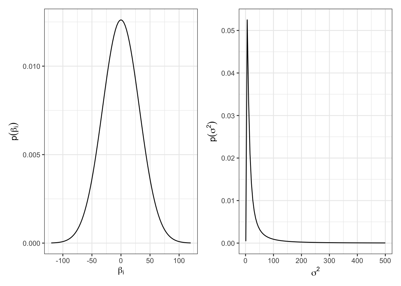
If we know very little about the relationships between \(X\) and \(\mathbf{y}\), we might wish to consider a “diffuse” prior that prescribes a large mass of uncertainty around each parameter.

math of prior
picture of prior

\[ \begin{aligned} \beta & \sim MVN(0, 1000 I)\\ 1/\sigma^2 &\sim \text{gamma}(1, 10) \end{aligned} \]

Sampler pseudo-code

pseudo-code

pick a starting \(\sigma^{2(0)}\), set \(s = 0\). Now for \(s\) in 1:S perform 1-3:
update \(\beta\):

compute \(V\) and \(\mathbf{m}\)
sample \(\beta^{(s+1)} \sim MVN(\mathbf{m}, V)\)

update \(\sigma^{2}\):

compute \(SSR(\beta^{(s+1)})\)
sample \(1/\sigma^{2(s+1)} \sim \text{gamma}([\nu_0 + n]/2, [\nu_0 \sigma_0^2 + SSR(\beta^{s+1})]/2)\)

save the states of \(\beta\) and \(\sigma^2\).

Code

The Gibbs sampler for our penguin example:

Code to reproduce penguins_subset

# our example examines just a subset of the penguin data
penguins_subset = penguins %>%
  select(body_mass_g, flipper_length_mm, bill_length_mm) %>%
  drop_na() %>%
  mutate(body_mass_kg = body_mass_g / 1000) %>%
  select(-body_mass_g)

X = penguins_subset %>%
  select(-body_mass_kg) %>%
  mutate(one = rep(1, nrow(penguins_subset))) %>%
  relocate(one) %>%
  as.matrix() 

y = select(penguins_subset, 
           body_mass_kg) %>%
  as.matrix()

set.seed(360)
# prior hyperparameters 
p = 2 # number of covariates
Sigma0 = 1000 * diag(rep(1, p+1)) # p + 1 for intercept term
b0 = rep(0, p + 1)
nu0 = 2
sigma02 = 10
n = nrow(y)

# starting values
## note: gamma = 1 / sigma^2
gamma = 1 / var(penguins_subset$body_mass_kg)

# values we should compute just once
SigmaInv = solve(Sigma0)
X2 = t(X) %*% X
Xy = t(X) %*% y
SIB0 = SigmaInv %*% b0
a = (nu0 + n) / 2
nu0s02 = nu0 * sigma02

## empty objects to fill
BETA = NULL
GAMMA = NULL

S = 2000
for (s in 1:S) {
  ### UPDATE BETA
  V = solve(SigmaInv + (gamma * X2))
  m = V %*% (Xy * gamma) # simplified since b0 = 0
  beta = rmvnorm(1, mean = m, sigma = V)
  
  ### UPDATE SIGMA
  SSR1 = (y - (X %*% t(beta)))
  SSRB = t(SSR1) %*% SSR1
  gamma = rgamma(1, a, ((nu0s02 + SSRB) / 2))
  
  ### SAVE STATES
  GAMMA = c(GAMMA, gamma)
  BETA = rbind(BETA, beta)
}

ESS?

effectiveSize(BETA)

var1 var2 var3 
2000 2000 2000

ESS?

effectiveSize(GAMMA)

var1 
2000

How do posterior mean estimates compare to the OLS estimates?

posteriorMean = apply(BETA, 2, mean)
OLS = lm(body_mass_kg ~ flipper_length_mm + bill_length_mm, data = penguins_subset) 
OLS = OLS$coefficients
rbind(OLS, posteriorMean)

              (Intercept) flipper_length_mm bill_length_mm
OLS             -5.736897        0.04814486    0.006047488
posteriorMean   -5.723741        0.04801443    0.006336029

We might have figured out this is what we were going to see already based on the the fact that the expressions for \(E[\beta | \mathbf{y}, X]\) and \(Var[\beta | \mathbf{y}, X]\) look just like \(E[\hat{\beta}_{OLS} | \beta]\) and \(Var[\hat{\beta}_{OLS} | \beta]\) when the prior information is diffuse.

What was the point of all that extra work? Well, we don’t just have a point estimate and a confidence interval, we have a whole posterior! We can quantify uncertainty about \(\beta\) in an easy and intuitive way.

Using the posterior, we may find 95% posterior CI, compute \(p(\beta_i > 0 | \mathbf{y}, X)\), compute \(p(\beta_i > \beta_j | \mathbf{y}, X)\), compute the posterior median, and a whole host of additional queries quickly and intuitively.

Let’s take a look at the marginal posteriors.

Exercise

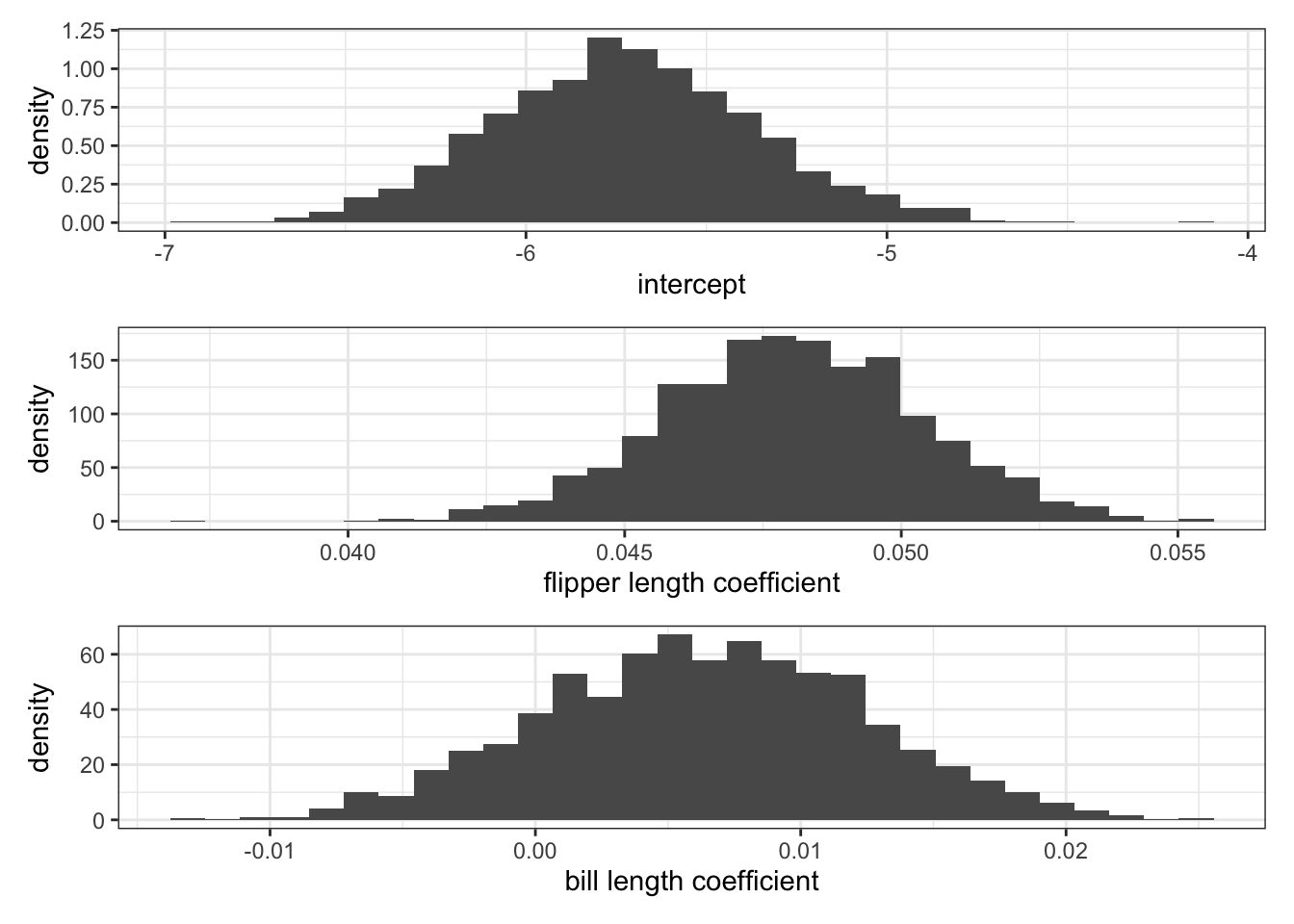
Is flipper length or bill length a “more important” predictor of penguin body mass? Why?

Visually

For each iteration of our Gibbs sampler, we’re sampling a hyperplane, i.e. a set of \(\beta\)s.

Exercise

Discuss how autocorrelation of \(\beta\)s would affect our sampler based on the animation above.

Other priors

Ridge regression and the normal prior

What if \(p > n\)? In words: what if we have more predictors than observations? \(X\) will be wide and therefore have linearly dependent columns.

In this case, \(X^T X\) is \(p \times p\) but is of rank \(n < p\), i.e. \(X^TX\) is not full rank and thus not invertible. Therefore, \(\hat{\beta}_{OLS}\) satisfying \((X^T X)\hat{\beta}_{OLS} = X^T \mathbf{y}\) does not exist uniquely.

Separately, in the case of multicollinearity, where the columns of \(X\) are highly correlated, some eigenvalues of \(X^TX\) will be very small, which means \((X^TX)^{-1}\) will have very large eigenvalues, i.e. \(Var(\hat{\beta}_{OLS})\) will be very large.

Intuitively: we can fix this by shrinking some of the \(\beta_i\) towards zero (reducing \(p\)).
Algebraically: one way we can fix this is by adding some positive quantity on the diagonals.

Frequentists call this sort of algebraic fix “ridge regression” and define the problem thus:

\[ \hat{\beta}_{ridge} = \underset{\beta}{\mathrm{argmin}} \underbrace{(\mathbf{y} - X\beta)^T (\mathbf{y} - X \beta)}_{\text{SSR}(\beta)} + \underbrace{\lambda \beta^T \beta}_{L_2^2 ~\text{penalty}} \] where \(\lambda\) is a tuning parameter called the “ridge coefficient”.

Bayesians obtain the same objective via the following prior on \(\beta\),

\[ \beta | \sigma^2, \lambda \sim MVN(0, \sigma^2 I /\lambda) \]

Exercise

Show that \(\hat{\beta}_{ridge} = E[\beta | \mathbf{y}, X, \sigma^2, \lambda] = ((X^TX) + \lambda I)^{-1} X^T \mathbf{y}\).