Multivariate normal

Author

Dr. Alexander Fisher

library(tidyverse)
library(mvtnorm) 
library(patchwork)

Visualizing a two-dimensional normal

Sigma = matrix(c(2, 0.7, 0.7, 1), 
               nrow = 2, ncol = 2)
mu = c(0, 0)

mu

[1] 0 0

Sigma

     [,1] [,2]
[1,]  2.0  0.7
[2,]  0.7  1.0

set.seed(360)
Y = rmvnorm(n = 500, 
        mean = mu,
        sigma = Sigma)

Y[1:5,]

           [,1]       [,2]
[1,]  2.0834251  0.7384787
[2,] -0.5817255 -1.0144046
[3,] -0.2769858 -0.7281417
[4,] -0.9446903 -0.3398126
[5,] -0.9972539  0.2615113

df = data.frame(y1 = Y[,1], y2 = Y[,2]) 
plot1 = df %>%
  ggplot(aes(x = y1, y = y2)) +
  geom_point() +
  theme_bw()
plot1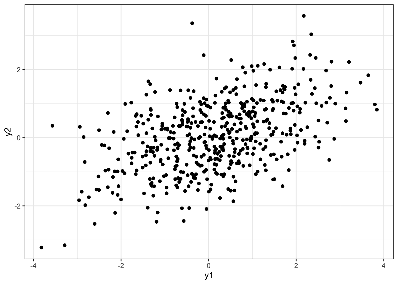

plot1 +
  geom_density_2d()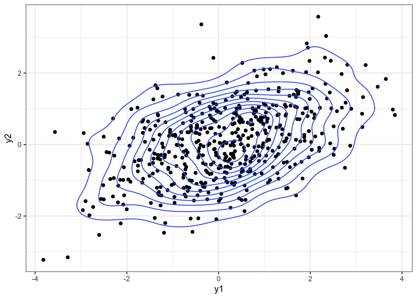

x = seq(-5, 5, 0.25) 
y = seq(-5, 5, 0.25)
f  = function(x, y) dmvnorm(cbind(x, y), mu, Sigma)
z = outer(x, y, f)
persp(x, y, z, theta = -30, phi = 25, 
      shade = 0.75, col = "steelblue", expand = 0.5, r = 2, 
      ltheta = 25, ticktype = "detailed", xlab ="y1",
      ylab = "y2",
      zlab = "")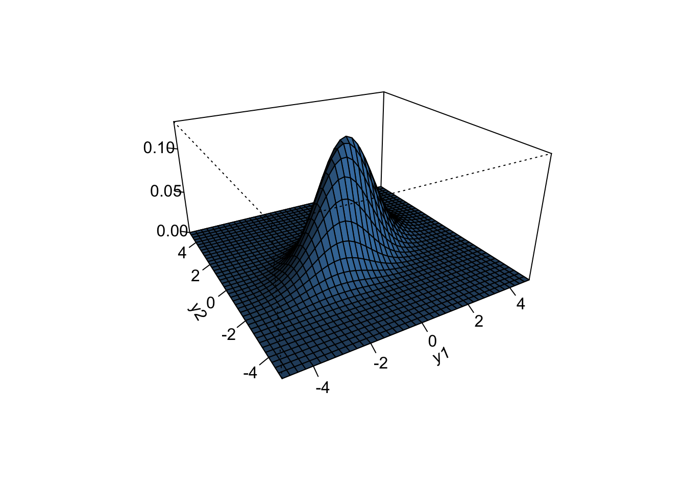

p1 = df %>%
  ggplot(aes(x = y1)) +
  geom_histogram(aes(y = ..density..)) +
  geom_density() +
  theme_bw()

p2 = df %>%
  ggplot(aes(x = y2)) +
  geom_histogram(aes(y = ..density..)) +
  geom_density() +
  theme_bw()

p1 + p2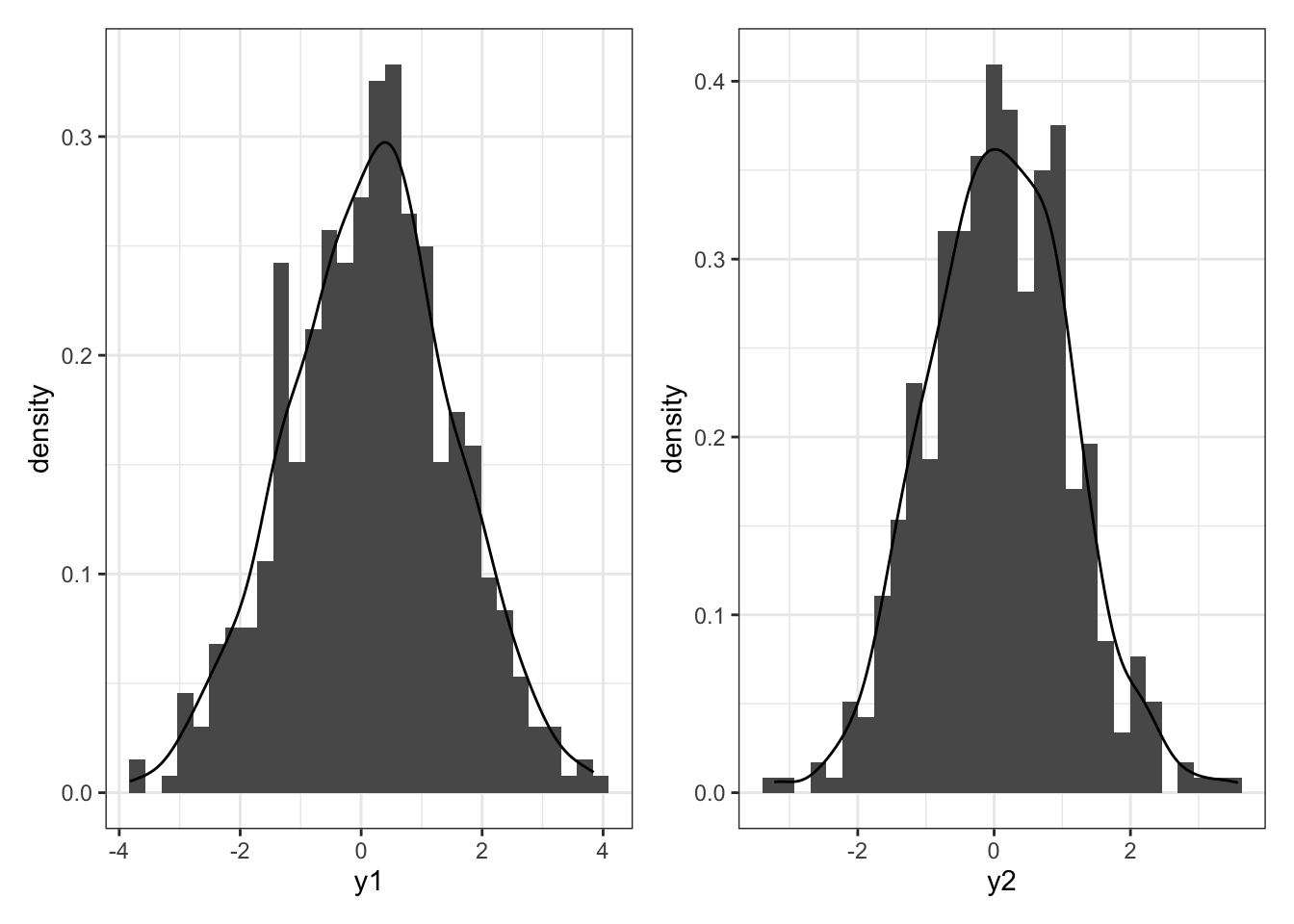

Density

We say a \(p\) dimensional vector \(\boldsymbol{Y}\) has a multivariate normal distribution if its sampling density is given by

\[ p(\boldsymbol{y}| \boldsymbol{\theta}, \Sigma) = (2\pi)^{-p/2} |\Sigma|^{-1/2} \exp\{ -\frac{1}{2}(\boldsymbol{y}-\boldsymbol{\theta})^T \Sigma^{-1} (\boldsymbol{y}- \boldsymbol{\theta}) \} \]

where

\[ \boldsymbol{y}= \left[ {\begin{array}{cc} y_1 \\ y_2\\ \vdots\\ y_p \end{array} } \right] ~~~ \boldsymbol{\theta}= \left[ {\begin{array}{cc} \theta_1 \\ \theta_2\\ \vdots\\ \theta_p \end{array} } \right] ~~~ \Sigma = \left[ {\begin{array}{cc} \sigma_1^2 & \sigma_{12}& \ldots & \sigma_{1p}\\ \sigma_{12} & \sigma_2^2 &\ldots & \sigma_{2p}\\ \vdots & \vdots & & \vdots\\ \sigma_{1p} & \ldots & \ldots & \sigma_p^2 \end{array} } \right]. \]

Key facts

\(\boldsymbol{y}\in \mathbb{R}^p\) ; \(\boldsymbol{\theta}\in \mathbb{R}^p\); \(\Sigma > 0\)
\(E[\boldsymbol{y}] = \boldsymbol{\theta}\)
\(V[\boldsymbol{y}] = E[(\boldsymbol{y}- \boldsymbol{\theta})(\boldsymbol{y}- \boldsymbol{\theta})^T] = \Sigma\)
Marginally, \(y_i \sim N(\theta_i, \sigma_i^2)\).
If \(\boldsymbol{\theta}\) is a MVN random vector, then the kernel is \(\exp\{-\frac{1}{2} \boldsymbol{\theta}^T A \boldsymbol{\theta}+ \boldsymbol{\theta}^T \boldsymbol{b} \}\). The mean is \(A^{-1}\boldsymbol{b}\) and the covariance is \(A^{-1}\).

sampling from a mvt norm

library(mvtnorm) contains functions we need.

rmvnorm() to sample from a multivariate normal
dmvnorm() to compute the density
pmvnorm() to compute the distribution function
qmvnorm() to compute quantiles of the multivariate normal

Matrix algebra fundamentals

matrix facts

matrix multiplication proceeds row \(\times\) column, so if we have the product \(AB\), \(A\) must have the same number of ___ as B has ___.
the determinant of a matrix, \(|A|\), measures the size of the matrix
the identity matrix is the matrix multiplicative identity. It is represented by \(\boldsymbol{I}\), in general \(\boldsymbol{I}_p\) is a \(p \times p\) matrix with 1 on each diagonal and 0 on every off-diagonal. \(\boldsymbol{I}A = A \boldsymbol{I}= A\).
the inverse of a matrix \(A^{-1}\) works as follows: \(A A^{-1} = A^{-1}A = \boldsymbol{I}\).
the trace of a matrix, tr(A), is the sum of its diagonal elements
order matters: \(AB \neq BA\) in general.
\(\Sigma > 0\) is shorthand for saying the matrix is positive definite. This means that for all vectors \(\boldsymbol{x}\), the quadratic form \(\boldsymbol{x}^T \Sigma \boldsymbol{x} > 0\). \(\Sigma > 0 \iff\) all eigenvalues of \(\Sigma\) are positive.

Exercise

\(\boldsymbol{\theta}\) and \(\boldsymbol{b}\) are \(p \times 1\) vectors, \(A\) is a symmetric matrix. Simplify \(\boldsymbol{b}^T A \boldsymbol{\theta}+ \boldsymbol{\theta}^T A \boldsymbol{b}\) what is the dimension of the result?
\(\boldsymbol{y}\) is a \(p \times 1\) vector. What’s the dimension of \(V[\boldsymbol{y}]\)?

matrix operations in R

# make a matrix A
A = matrix(c(1,.2, .2, 2), ncol = 2)
A

     [,1] [,2]
[1,]  1.0  0.2
[2,]  0.2  2.0

# invert A (expensive for large matrices)
Ainv = solve(A)

# matrix multiplication
Ainv %*% A

     [,1] [,2]
[1,]    1    0
[2,]    0    1

# determinant of A
det(A)

[1] 1.96

# trace of A
sum(diag(A))

[1] 3

# create a vector b
b = matrix(c(1, 2), ncol = 1)
b

     [,1]
[1,]    1
[2,]    2

# transpose the vector b
t(b)

     [,1] [,2]
[1,]    1    2

b %*% A

Error in b %*% A: non-conformable arguments

What went wrong in the code above?

Semiconjugate priors

Definition

A semiconjugate or conditionally conjugate prior is a prior that is conjugate to the full conditional posterior.

semiconjugate prior for \(\boldsymbol{\theta}\)

\[ \begin{aligned} \boldsymbol{y}| \boldsymbol{\theta}, \Sigma &\sim MVN(\boldsymbol{\theta}, \Sigma),\\ \boldsymbol{\theta}&\sim MVN(\mu_0, \Lambda_0), \end{aligned} \]

then

\[ \boldsymbol{\theta}| \boldsymbol{y}, \Sigma \sim MVN(\boldsymbol{\mu_n}, \Lambda_n), \]

where

\[ \begin{aligned} \Lambda_n &= (\Lambda_0^{-1} + n \Sigma^{-1} )^{-1},\\ \boldsymbol{\mu_n} &= (\Lambda_0^{-1} + n \Sigma^{-1} )^{-1}(\Lambda_0^{-1} \boldsymbol{\mu}_0 + n \Sigma^{-1} \bar{\boldsymbol{y}}). \end{aligned} \]

Exercise

Interpret \(E[\boldsymbol{\theta}| \boldsymbol{y}_1, \ldots \boldsymbol{y}_n, \Sigma]\) and \(Cov[\boldsymbol{\theta}| \boldsymbol{y}_1, \ldots \boldsymbol{y}_n, \Sigma]\).

semiconjugate prior for \(\Sigma\)

\[ \begin{aligned} \boldsymbol{y}| \boldsymbol{\theta}, \Sigma &\sim MVN(\boldsymbol{\theta}, \Sigma),\\ \Sigma &\sim \text{inverse-Wishart}(\nu_0, S_0^{-1}), \end{aligned} \]

then

\[ \Sigma | \boldsymbol{y}, \boldsymbol{\theta}\sim \text{inverse-Wishart} (\nu_0 + n, (S_0 + S_{\theta})^{-1}), \] where \(S_\theta = \sum_{i=1}^n (\boldsymbol{y}_i - \boldsymbol{\theta})(\boldsymbol{y}_i - \boldsymbol{\theta})^T\) is the residual sum of squares matrix for the vectors \(\boldsymbol{y}_1, \ldots \boldsymbol{y}_n\) if the population mean is \(\boldsymbol{\theta}\).

the inverse-Wishart

the inverse-Wishart\((\nu_0, S_0^{-1})\) density is given by

\[ \begin{aligned} p(\Sigma | \nu_0, S_0^{-1}) = \left[ 2^{\nu_0 p / 2} \pi^{{p \choose 2}/2} |S_0|^{-\nu_0/2} \prod_{j = 1}^p \Gamma([\nu_0 + 1 - j]/2) \right]^{-1} \times\\ |\Sigma|^{-(\nu_0 + p + 1)/2} \times \exp \{ -\frac{1}{2}tr(S_0 \Sigma^{-1})\}. \end{aligned} \]

Key facts

notice that the first line is the normalizing constant of the density
the support is \(\Sigma > 0\) and \(\Sigma\) symmetric \(p \times p\) matrix. \(\nu_0 \in \mathbb{N}^+\) and \(\nu_0 \geq p\). \(S_0\) is a \(p \times p\) symmetric positive definite matrix.
if \(\Sigma\) is inv-Wishart\((\nu_0, S_0^{-1})\) then \(\Sigma^{-1}\) is Wishart\((\nu_0, S_0^{-1})\).
\(E[\Sigma^{-1}] = \nu_0 S_0^{-1}\) and \(E[\Sigma] = \frac{1}{\nu_0 - p - 1} S_0\).
intuition: \(\nu_0\) is prior sample size. \(S_0\) is a prior guess of the covariance matrix.

sampling from the inverse-Wishart

pick \(\nu_0 > p\), pick \(S_0\)
sample \(\boldsymbol{z}_1, \ldots \boldsymbol{z}_{\nu_0} \sim \text{ i.i.d. } MVN(\boldsymbol{0}, S_0^{-1})\)
calculate \(\boldsymbol{Z}^T \boldsymbol{Z} = \sum_{i = 1}^{\nu_0} \boldsymbol{z}_i \boldsymbol{z}^T\)
set \(\Sigma = (\boldsymbol{Z}^T \boldsymbol{Z})^{-1}\)

library(mvtnorm) # contains function rmvnorm

# 2x2 example: generating 1 sample from an inv-Wishart
set.seed(360)
p = 2
nu0 = 3
S0 = matrix(c(1, .1, .1, 1), ncol = 2)
S0inv = solve(S0)
Z = rmvnorm(n = nu0, # number of observations of the 2D vector Z
        mean = rep(0, p), # mean 0
        sigma = S0inv) # prior variance
Sigma = solve(t(Z) %*% Z)
eigen(Sigma)$values

[1] 0.7821737 0.4174527

Sigma

           [,1]      [,2]
[1,]  0.5271834 -0.167273
[2,] -0.1672730  0.672443

Exercise

Why does this work? Hint: what is \(Var[\boldsymbol{z}]\)?

We can also use the monomvn package to simulate from a Wishart more succinctly,

library(monomvn)

set.seed(360)
Sigma = solve(rwish(nu0, S0inv))
eigen(Sigma)$values

[1] 0.692529 0.160428

Sigma

          [,1]      [,2]
[1,] 0.1899212 0.1217519
[2,] 0.1217519 0.6630358