The normal model

Author

Dr. Alexander Fisher

# load packages
library(tidyverse)
library(latex2exp)

Background

Definition and vocabulary

Let \(Y\) be normally distributed with mean \(\theta\) and variance \(\sigma^2\). Mathematically,

\[ Y | \theta, \sigma^2 \sim N(\theta, \sigma^2). \] The density \[ \begin{aligned} p(y ~|~ \theta, \sigma^2 ) &= (2\pi\sigma^2)^{-1/2} e^{-\frac{1}{2\sigma^2} (y-\theta)^2},\\ y &\in \mathbb{R},\\ \theta &\in \mathbb{R},\\ \sigma &\in \mathbb{R}^+. \end{aligned} \]

location, scale

\(\theta\) is called the ‘location’ parameter
\(\sigma\) is called the ‘scale’ parameter

precision

Notice that every time \(\sigma^2\) appears in the density, it is inverted. For this reason, the inverse variance \((\frac{1}{\sigma^2})\) has a special name, precision. Intuitively, precision tells us how close \(y\) is to the mean \(\theta\). (Large precision = small variance = closer).

plots of normal densities

Warning

In R, the arguments of pnorm, dnorm, rnorm are the mean and standard deviation (not the variance!)

plot
code

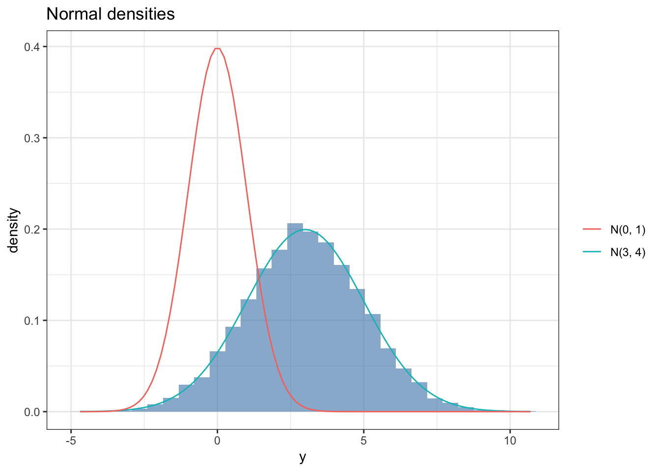
set.seed(123)
N = 10000
y.mc = rnorm(N, mean = 3, sd = 2)

df = data.frame(y.mc)

df %>%
  ggplot(aes(x = y.mc)) +
  geom_histogram(aes(y = ..density..), alpha = 0.6, fill = 'steelblue') +
  stat_function(fun = dnorm, args = list(mean = 3, sd = 2), aes(color = "N(3, 4)")) +
  stat_function(fun = dnorm, args = list(mean = 0, sd = 1), aes(color = "N(0, 1)")) +
  theme_bw() +
  labs(x = "y", y = "density", title = "Normal densities",
       color = "")

Bayesian inference

In general, we wish to make inference about \(\theta\) and \(\sigma^2\) after observing some data \(y_1, \ldots y_n\) and thus are interested in the posterior \(p(\theta, \sigma^2 | y_1, \ldots y_n)\). This is the standard task we have seen thus far, and requires us to specify a joint prior \(p(\theta, \sigma^2)\). Below, we will work to find a class of conjugate priors over \(\theta\) and \(\sigma^2\).

We can break up the joint posterior into two pieces from the axioms of probability:

\[ p(\theta, \sigma^2 | y_1, \ldots y_n) = p(\theta | \sigma^2, y_1, \ldots, y_n)p(\sigma^2|y_1, \ldots y_n) \] This suggests that we calculate the joint posterior by:

first finding the full conditional of \(\theta\): \(p(\theta| \sigma^2, \vec{y})\)
and then finding the marginal posterior of \(\sigma^2\): \(p(\sigma^2 | \vec{y})\),

where \(\vec{y} = \{y_1, \ldots y_n\}\).

The full conditional of \(\theta\)

By Bayes’ theorem,

\[ p(\theta| \sigma^2, \vec{y}) \propto \underbrace{p(\vec{y} |\theta, \sigma^2)}_{\text{likelihood}} \underbrace{p(\theta|\sigma^2)}_{\text{prior}}. \] To arrive at the full conditional posterior of \(\theta\), we must first specify a prior on \(\theta\).

Considering we have a normal likelihood, what is a conjugate class of densities for \(\theta\)?

answer

\(\theta | \sigma^2 \sim N(\mu_0, \tau_0^2)\) for some \(\mu_0 \in \mathbb{R}\) and \(\tau_0^2 \in \mathbb{R}^+\) is conjugate.

With the conjugate prior, our full conditional posterior \(\{ \theta| \sigma^2, \vec{y} \} \sim N(\mu_n, \tau_n^2)\) where

\[ \begin{aligned} \mu_n &= \frac{\frac{1}{\tau_0^2}\mu_0 + \frac{n}{\sigma^2} \bar{y}}{ \frac{1}{\tau_0^2} + \frac{n}{\sigma^2} } \\ \\ \tau_n^2 &= \frac{1}{\frac{1}{\tau_0^2} + \frac{n}{\sigma^2}} \end{aligned} \]

Let’s sketch out ‘completing the square’ to derive the parameters offline.

Intuitive posterior parameters

If we consider the posterior precision, \(\frac{1}{\tau_n^2}\), we can re-arrange the terms above to illuminate how posterior information = prior information + data information;.

\[ \frac{1}{\tau_n^2}= \frac{1}{\tau_0^2} + \frac{n}{\sigma^2} \] In words, posterior precision is equivalent to prior precision plus sampling precision. If we name each precision term, \(\lambda_0 = \frac{1}{\tau_0}\) and \(\lambda = \frac{1}{\sigma}\) then

\[ \mu_n = \frac{\lambda_0^2}{\lambda_0^2 + n\lambda^2} \mu_0 + \frac{n\lambda^2}{\lambda_0^2 + n\lambda^2} \bar{y} \]

i.e. the posterior mean is the weighted average of prior and sample mean, where the weights are the relative contribution of each precision!

We can re-define \(\lambda_0^2 = \kappa_0 \lambda^2\) (or equivalently \(\tau_0^2 = \frac{\sigma^2}{\kappa_0}\)) and obtain

\[ \begin{aligned} \mu_n &= \frac{\kappa_0}{\kappa_0 + n} \mu_0 + \frac{n}{\kappa_0 + n} \bar{y},\\ \frac{1}{\tau_n^2} &= \frac{\kappa_0 + n}{\sigma^2} \end{aligned} \]

where we can interpret \(\kappa_0\) as the prior sample size.

Important

Note that \(\tau_n^2\) is the posterior variance of the full conditional posterior of \(\theta\). This is distinct from \(\sigma_n^2\), defined below.

Prior on \(\sigma^2\)

Remember, we want \(p(\theta, \sigma^2 | \vec{y}) = p(\theta | \sigma^2, y_1, \ldots, y_n)p(\sigma^2|y_1, \ldots y_n)\). We have the first component of the right hand side, what about the second component?

Notice that

\[ p(\sigma^2 | \vec{y}) \propto p(\sigma^2)\int p(\vec{y} | \theta, \sigma^2) p(\theta|\sigma^2) d\theta \]

But how do we choose \(p(\sigma^2)\) to be conjugate? We can proceed in multiple ways: one is noting that the integral is really a convolution of normals, (thereby a sum of normals) and is therefore a normal density.

Upon inspection, we can see a suitable choice is \(\frac{1}{\sigma^2} \sim \text{gamma}(a, b)\).

The inverse-gamma

A random variable \(X \in (0, \infty)\) has an inverse-gamma(a,b) distribution if \(\frac{1}{X}\) has a gamma(a,b) distribution.

If X has an inverse-gamma distribution, the density of X is

\[ p(x | a, b) = \frac{b^a}{\Gamma(a)} x^{-a-1}e^{-b/x} \ \text{for } \ x > 0 \] and \[ \begin{aligned} EX &= \frac{b}{(a-1)} \text{ if } a \geq 1; \ \infty \text{ if } 0<a<1,\\ Var(X) &= \frac{b^2}{(a-1)^2(a-2)} \ \text{if } a \geq 2; \ \infty \text{ if } 0 < a < 2,\\ Mode(X) &= \frac{b}{a +1}. \end{aligned} \]

The marginal posterior of \(\sigma^2\)

Taken all together, if we let our sampling model and prior distributions be such that \[ \begin{aligned} Y_i | \theta, \sigma^2 &\sim N(\theta, \sigma^2)\\ \theta | \sigma^2 & \sim N(\mu_0, \sigma^2/\kappa_0)\\ \frac{1}{\sigma^2} &\sim \text{gamma}(\frac{\nu_0}{2}, \frac{\nu_0}{2} \sigma_0^2) \end{aligned} \] then the posterior

\[ \frac{1}{\sigma^2} | \vec{y} \sim \text{gamma}(\frac{\nu_n}{2}, \frac{\nu_n \sigma^2_n}{2}), \] where \[ \begin{aligned} \nu_n &= \nu_0 + n,\\ \sigma^2_n &= \frac{1}{\nu_n} \left[ \nu_0 \sigma^2_0 +(n-1)s^2 + \frac{\kappa_0 n}{\kappa_0 + n}(\bar{y} - \mu_0)^2 \right], \end{aligned} \]

and \(s^2\) is the sample variance, \(\frac{1}{n-1} \sum_i (y_i - \bar{y})^2\).

Sampling from the joint posterior

Since \(p(\theta, \sigma^2 | \vec{y}) = p(\theta | \sigma^2, y_1, \ldots, y_n)p(\sigma^2|y_1, \ldots y_n)\), we can sample from the joint posterior by first sampling from \(p(\sigma^2|y_1, \ldots y_n)\) and then sampling from \(p(\theta | \sigma^2, y_1, \ldots, y_n)\).

Example

Proof of concept

We have some data:

# generating 10 samples from the population
set.seed(123)
true.theta = 4
true.sigma = 1
y = rnorm(10, true.theta, true.sigma)

ybar = mean(y) # sample mean
n = length(y) # sample size
s2 = var(y) # sample variance

We make inference about \(\theta\) and \(\sigma^2\):

# priors
# theta prior
mu_0 = 2; k_0 = 1
# sigma2 prior
nu_0 = 1; s2_0 = 0.010

# posterior parameters
kn = k_0 + n
nun = nu_0 + n
mun = (k_0 * mu_0 + n * ybar) /kn
s2n = (nu_0 * s2_0 + (n - 1) * s2 + k_0 * n * (ybar - mu_0)^2 / (kn)) / (nun)

s2.postsample = 1 / rgamma(10000, nun / 2, s2n * nun / 2)
theta.postsample = rnorm(10000, mun, sqrt(s2.postsample / kn))

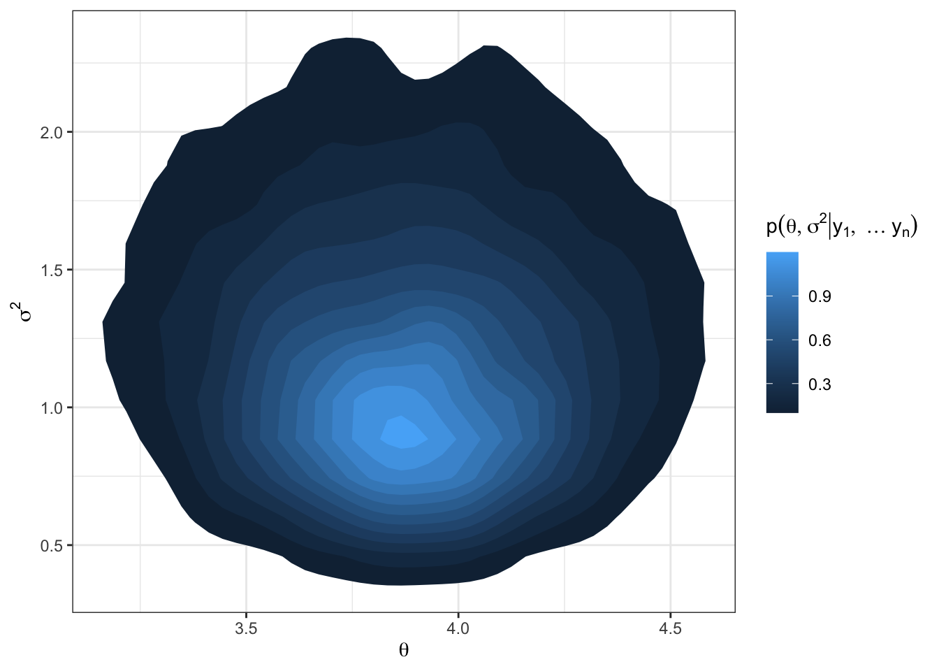
df = data.frame(theta.postsample, s2.postsample)

df %>%
  ggplot(aes(x = theta.postsample, y = s2.postsample)) +
  stat_density_2d(aes(fill = ..level..), geom = "polygon") +
  labs(x = TeX("$\\theta$"),
       y = TeX("$\\sigma^2$"),
       fill = TeX("$p(\\theta, \\sigma^2 | y_1, \\ldots y_n)$")) +
  theme_bw()