library(tidyverse)
library(latex2exp)Intro to Monte Carlo
Load packages:
Monte Carlo motivation
General social survey from the 90s gathered data on the number of children to women of two categories: those with and without a bachelor’s degree.
Setup:
- \(Y_{i1}\): number of children of \(i\)th woman in group 1 (no bachelor’s)
- \(Y_{i2}\): number of children of \(i\)th woman in group 2 (bachelor’s)
Model:
- \(Y_{11}, \ldots, Y_{n_1 1} | \theta_1 \overset{\mathrm{iid}}{\sim} \text{Poisson}(\theta_1)\)
- \(Y_{12} \ldots, Y_{n_2 2} | \theta_2 \overset{\mathrm{iid}}{\sim} \text{Poisson}(\theta_2)\)
Prior:
- \(\theta_1 \sim \text{gamma}(2, 1)\)
- \(\theta_2 \sim \text{gamma}(2, 1)\)
Data:
- \(n_1 = 111\), \(\bar{y_1} = 1.95\), \(\sum y_{i 1} = 217\)
- \(n_2 = 44\), \(\bar{y_1} = 1.5\), \(\sum y_{i 1} = 66\)
Posterior:
- \(\theta_1 | \vec{y_1} \sim \text{gamma}(219, 112)\)
- \(\theta_2 | \vec{y_2} \sim \text{gamma}(68, 45)\)
We already know how to compute
- posterior mean: \(E~\theta | y = \alpha / \beta\) (shape, rate parameterization)
- posterior density (
dgamma) - posterior quantiles and confidence intervals (
qgamma)
What about posterior distribution of \(|\theta_1 - \theta_2|\), \(\theta_1 / \theta_2\), \(\text{max} \{\theta_1, \theta_2 \}\)?
What about the probability a woman with a bachelor’s has more children than a woman without a bachelors? \(p(\tilde{y}_1 < \tilde{y}_2 | \vec{y_1}, \vec{y_2})\)?
Monte Carlo integration
- approximates an integral by a stochastic average
- shines when other methods of integration are impossible (e.g. high dimensional integration)
- works because of law of large numbers: for a random variable \(\theta\), the sample mean \(\bar{\theta}_N\) converges to the true mean \(\mu\) as the number of samples \(N\) tends to infinity.
The key idea is: we obtain independent samples from the posterior,
\[ \theta^{(1)}, \ldots \theta^{(N)} \overset{\mathrm{iid}}{\sim} p(\theta |\vec{y}) \] then the empirical distribution of the samples approximates the posterior (approximation improves as \(N\) increases).
Recall
\[ E~g(\theta)|y = \int_\mathcal{\theta} g(\theta) p(\theta | y)d\theta \approx \frac{1}{N} \sum_{i = 1}^N g(\theta^{(i)}). \]
The law of large numbers says that if our samples \(\theta^{(i)}\) are independent, \(\frac{1}{N} \sum_{i = 1}^N g(\theta^{(i)})\) converges to \(E~g(\theta)|y\).
Note
Integrals are expectations, and expectations are integrals.
Examples
- \(\theta_1 | \vec{y_1} \sim \text{gamma}(219, 112)\)
- \(\theta_2 | \vec{y_2} \sim \text{gamma}(68, 45)\)
(1) proof of concept: the mean
set.seed(123)
N = 5000
rgamma(N, shape = 219, rate = 112) %>%
  mean()
[1] 1.95294Pretty close to the true mean, 1.9553571.
(2) posterior of \(|\theta_1 - \theta_2|\)
set.seed(123)
theta1 = rgamma(N, shape = 219, rate = 112)
theta2 = rgamma(N, shape = 68, rate = 45)

df = data.frame(diff = abs(theta1 - theta2))

df %>%
  ggplot(aes(x = diff)) +
  geom_density() +
  theme_bw() +
  labs(x = TeX("$|\\theta_1 - \\theta_2|$"),
       y = TeX("$p(|\\theta_1 - \\theta_2 || {y}_1, {y}_2)$"))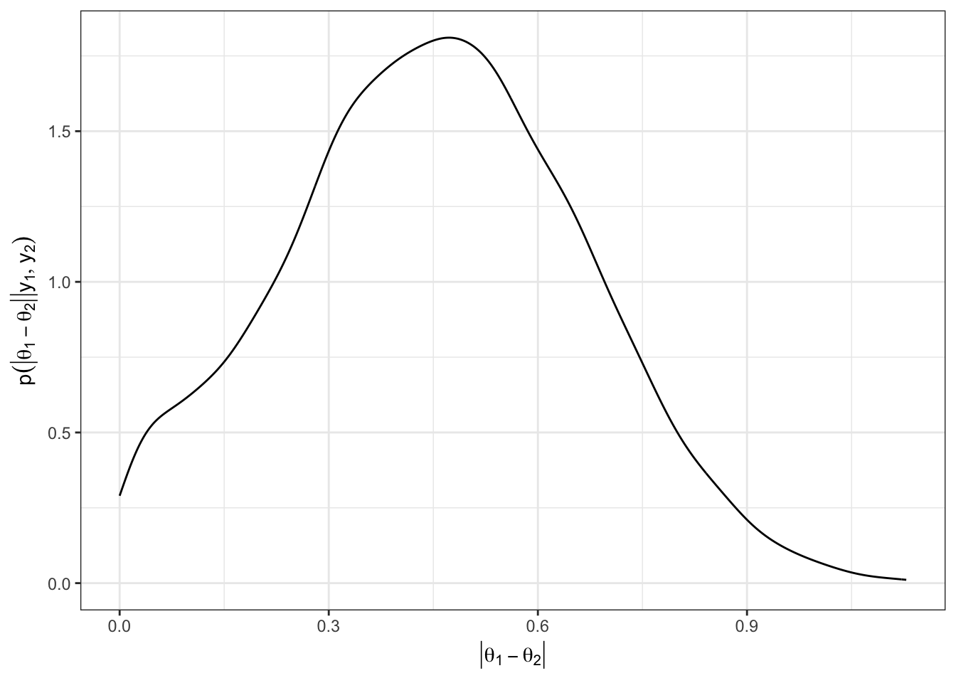
(3) \(p(|\theta_1 - \theta_2|> .5)\)
mean(df$diff > .5)[1] 0.4108
Exercise
- \(\theta \sim \text{uniform}(0, 2)\)
- Let \(\phi = \log \theta\)
- Visualize \(p(\phi)\) using Monte Carlo simulation, then show using the change of variables formula and plotting the closed form of the density.
# sample from p(theta)
theta = runif(10000, 0, 2)

# define transform function
f = function(x) {
  return(0.5 *exp(x))
}

# create a df for each plot
df = data.frame(phi = -7:0)
df2 = data.frame(phiSamples = log(theta))

# make plots
df %>%
  ggplot(aes(x = phi)) +
  stat_function(fun = f, col = 'red', alpha = 0.5) +
  geom_histogram(data = df2, aes(x = phiSamples,
                                 y = ..density..),
               fill = 'steelblue', alpha = 0.5)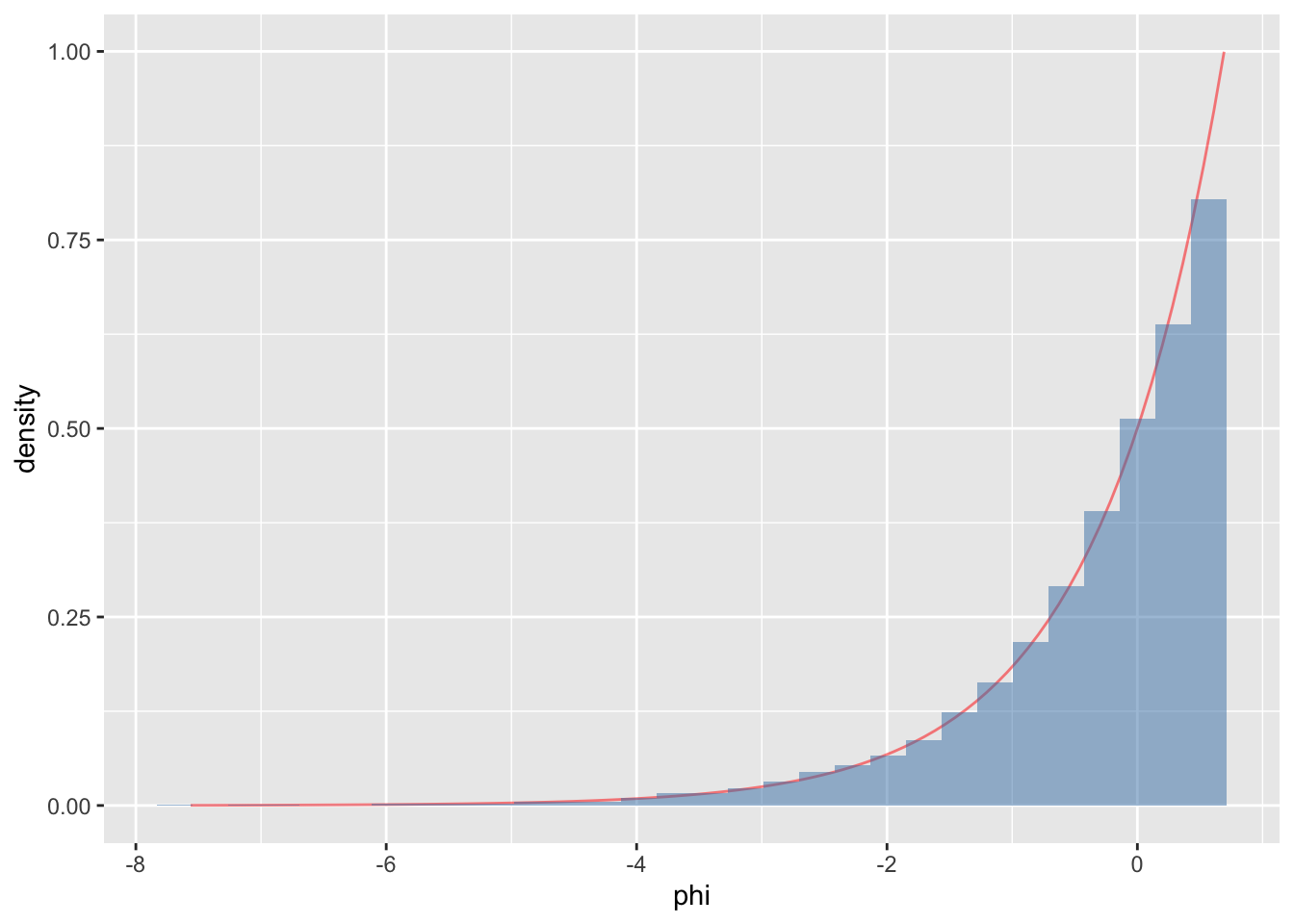
# Just making the Monte Carlo part of the plot
# in 3 lines
theta = runif(10000, 0, 2)
phi = log(theta)
hist(phi)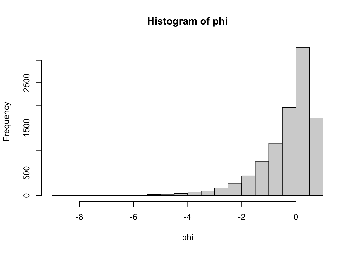
Exercise
What is \(Pr(\tilde{y}_1 < \tilde{y}_2 | \vec{y_1}, \vec{y_2})\)?
theta1 = rgamma(N, shape = 219, rate = 112)
theta2 = rgamma(N, shape = 68, rate = 45)

y1tilde = rpois(N, theta1)
y2tilde = rpois(N, theta2)

# y1: no. children to parent w/ no bachelors
# y2: no. children to parent w/ bachelors
mean(y1tilde < y2tilde)
[1] 0.307