Posterior summaries and reliability

library(tidyverse)
library(latex2exp)

Confidence regions

Bayesian confidence interval

Definition

Let \(\Phi\) be the support of \(\theta\). An interval \((l(y), u(y)) \subset \Phi\) has \(100 \times (1-\alpha)\%\) posterior coverage if

\[ p(l(y) < \theta < u(y) | y ) = (1-\alpha) \]

Interpretation: after observing \(Y = y\), our probability that \(\theta \in (l(y), u(y))\) is \(100 \times (1-\alpha)\%\).

If \(\alpha = 0.05\), such an interval is called 95% posterior confidence interval (CI). It may also sometimes be referred to as a 95% “credible interval” to distinguish it from a frequentist CI.

Important

This is a probability statement about \(\theta\)!

Frequentist confidence interval

Contrast posterior coverage to frequentist coverage:

Definition

A random interval \((l(Y), u(Y)\)) has 95% frequentist coverage for \(\theta\) if before data are observed,

\[ p(l(Y) < \theta < u(Y) | \theta) = 0.95 \]

Interpretation: if \(Y \sim P_\theta\) then the probability that \((l(Y), u(Y)\) will cover \(\theta\) is 0.95.

In practice, for many applied problems

\[ p(l(y) < \theta < u(y) | y ) \approx p(l(Y) < \theta < u(Y) | \theta) \]

see section 3.1.2. in the book.

Example: posterior CI for beta-binomial

Let \(Y_1, \ldots Y_n\) be binary random variables that are conditionally independent given \(\theta\) so that \(p(y_i | \theta) = \theta^{y_i} (1-\theta)^{1-y_i}\). Let \(\theta \sim beta(a, b)\).

Recall that \(\theta | y_1,\ldots y_n \sim beta(a + \sum{y_i}, b + n - \sum y_i)\).

Therefore, a \((1-\alpha)\) confidence interval can be computed for a given \(a, b\) and data \(n, \sum y_i\), see coded example below:

a = 6
b = 6
sumY = 8
n = 10

posteriorMean = (a + sumY) / (a + b + n)

alpha = 0.05
lower_q = alpha / 2
upper_q = 1 - (alpha / 2)
theta_ci_95  = qbeta(p = c(lower_q, upper_q), a + sumY, b + n - sumY)

The posterior mean \(E[\theta | y_1,\ldots y_n] =\) 0.64 with 95% Bayesian CI (0.43,0.82).

plot

code

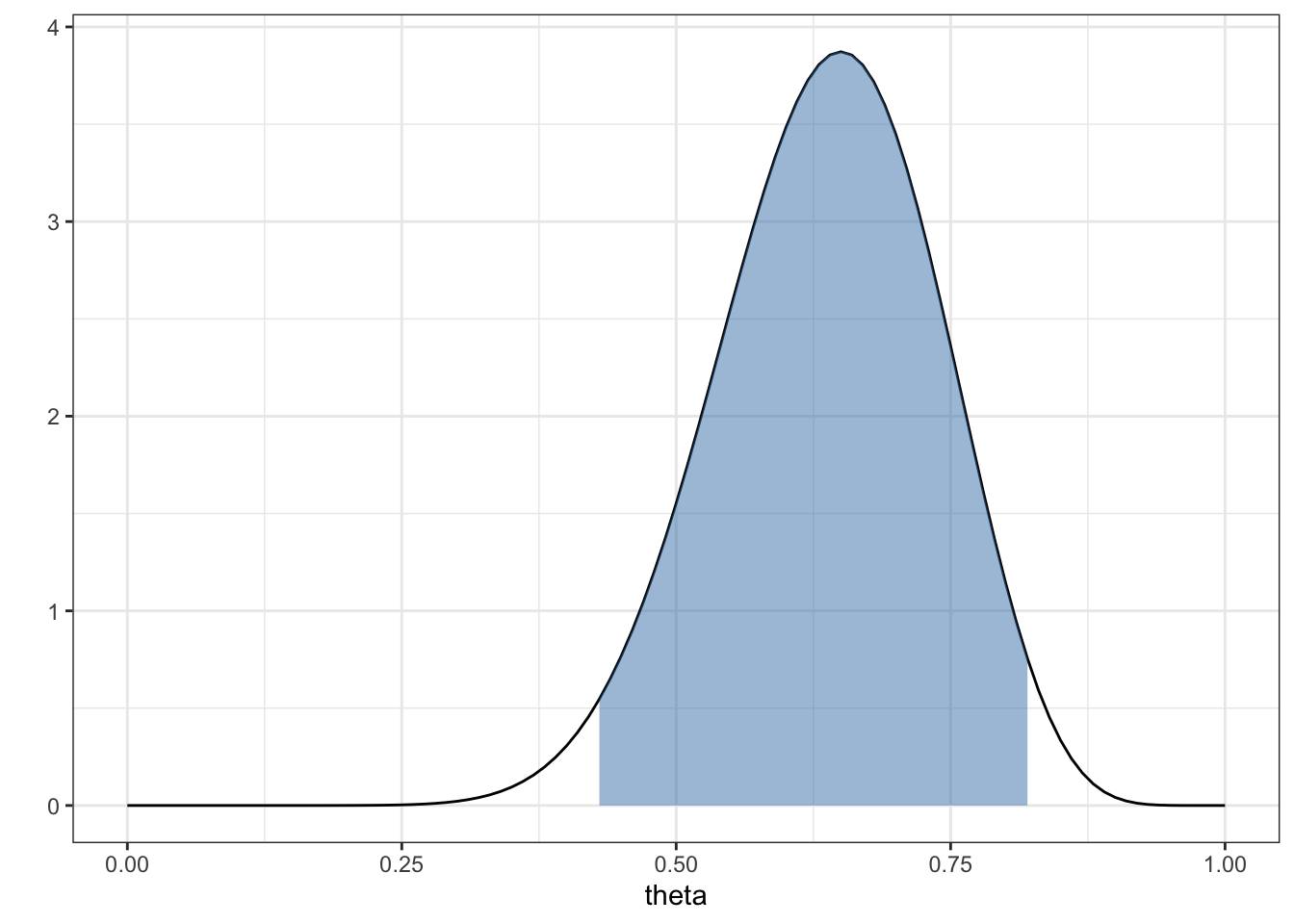
data.frame(theta = c(0, 1)) %>%
  ggplot(aes(x = theta)) + 
  stat_function(fun = dbeta, args = list(a + sumY, b + n - sumY)) + 
  theme_bw() +
  labs(y = "") +
  geom_area(stat = "function", fun = dbeta, args = list(a + sumY, b +n - sumY),
            fill = "steelblue", xlim = theta_ci_95, alpha = 0.5)

High posterior density

Definition

A \(100 \times (1-\alpha)\)% high posterior density (HPD) region is a set \(s(y) \subset \Theta\) such that

1. \(p(\theta \in s(y) | Y = y) = 1 - \alpha\)

2. If \(\theta_a \in s(y)\) and \(\theta_b \not\in s(y)\), then \(p(\theta_a | Y = y) > p(\theta_b | Y = y)\)

• Note: all points inside an HPD region have higher posterior density than points outside the region.
• Note: the HPD region is not always an interval.

Example: HPD for a mixture of normals

Laplace approximation

Posterior mode: sometimes called “MAP” or “maximum a posteriori” estimate, this quantity is given by \(\hat{\theta} = \arg \max_{\theta} p(\theta | y)\).

• Notice this unwinds to be \(\hat{\theta} = \arg \max_{\theta} p(y | \theta) p(\theta)\).

One way to report the reliability of the posterior mode is to look at the width of the posterior near the mode, which we can sometimes approximate with a Gaussian distribution:

\[ p(\theta | y) \approx C e^{\frac{1}{2} \frac{d^2L}{d\theta^2}|_{\hat{\theta}} (\theta - \hat{\theta})^2} \] where \(C\) is a normalization constant and \(L\) is the log-posterior, \(\log p(\theta | y)\).

Taken together, the fitted Gaussian with a mean equal to the posterior mode is called the Laplace approximation.

• Let’s derive the Laplace approximation offline

Exercise

For the beta-binomial model above, compute the Laplace approximation.

plot

code

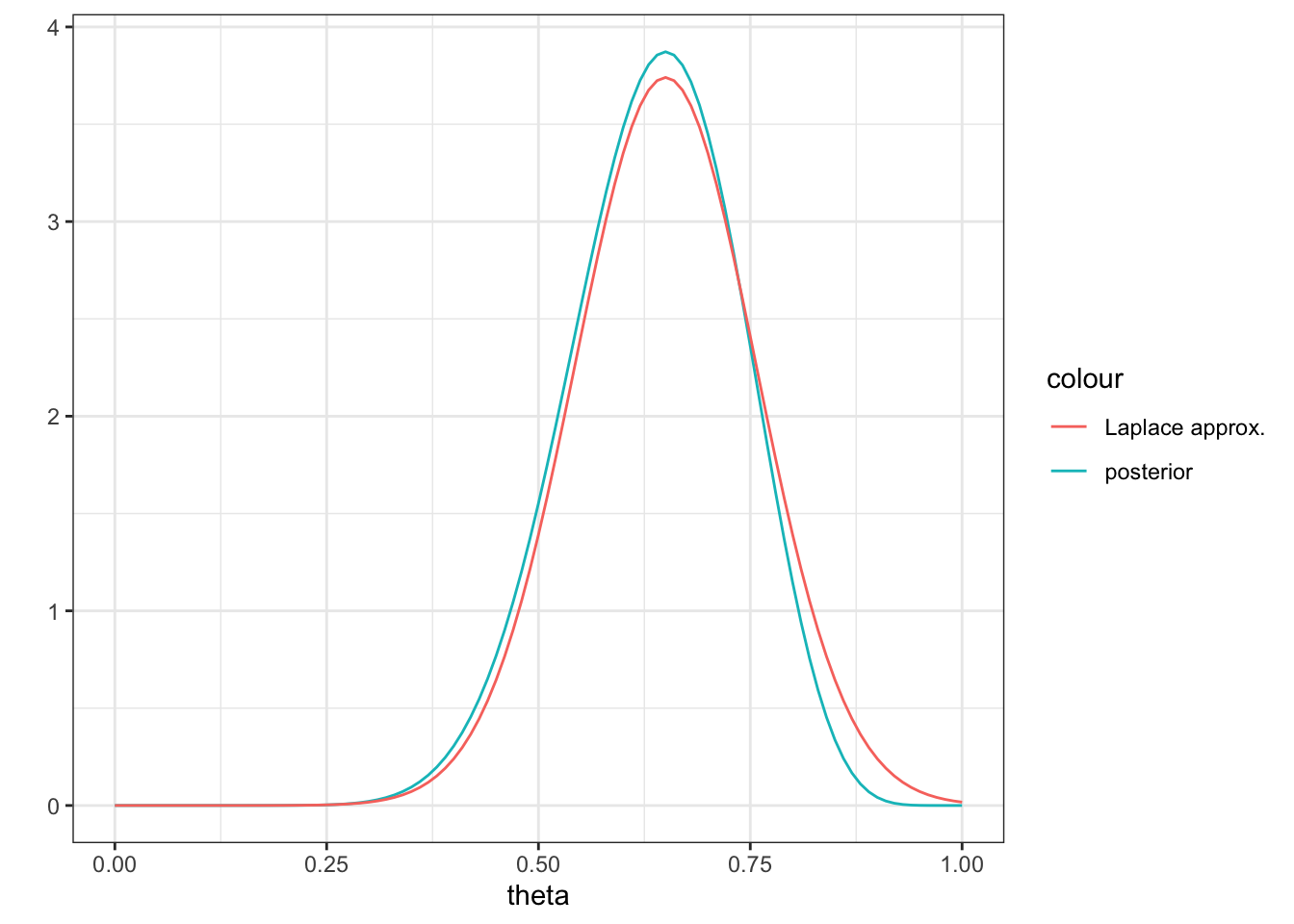
alpha = a + sumY
beta = b + n - sumY

d2posterior = function(theta) {
  ( (1-alpha) / (theta^2) ) - 
    ((beta - 1) / (1 - theta)^2)
}

thetaHAT = (alpha - 1) / (beta - 2 + alpha)
sdhat = sqrt(- 1 / d2posterior(thetaHAT))

data.frame(theta = c(0, 1)) %>%
  ggplot(aes(x = theta)) + 
  stat_function(aes(color = "posterior"),
                fun = dbeta, args = list(alpha, beta)) + 
  theme_bw() +
  labs(y = "") +
  stat_function(aes(color = "Laplace approx."), fun = dnorm,
                args = list(mean = thetaHAT, sd = sdhat))