See libraries used in these notes
library(tidyverse)
library(latex2exp)library(tidyverse)
library(latex2exp)In basketball, an “assist” is attributed to a player that passes the ball to a teammate in a way that directly leads to a basket. The data below was scraped from espn.com September 2024. Each row of the data set is an individual Boston Celtics player during a particular game of the 2023-2024 season. The AST records the number of assists made by the player in the particular game. MIN records the number of minutes each player played in a particular game. vs records the opposing team.
# A tibble: 10 × 4
   player                 AST   MIN vs
   <chr>                <dbl> <dbl> <chr>
 1 Payton Pritchard PG      4  23.5 Golden State Warriors
 2 Derrick White PG         4  33.5 Dallas Mavericks
 3 Jaylen Brown SG          4  34   Brooklyn Nets
 4 Luke Kornet C            2  21.3 Chicago Bulls
 5 Xavier Tillman F *       2  15   Dallas Mavericks
 6 Luke Kornet C            1  19   Dallas Mavericks
 7 Kristaps Porzingis C     1  23.7 Brooklyn Nets
 8 Kristaps Porzingis C     1  30   Chicago Bulls
 9 Oshae Brissett SF        0   4   Dallas Mavericks
10 Luke Kornet C 0 11 Golden State Warriorsset.seed(360)
yx = read_csv("../data/BostonCeltics_Assists_23-24_season.csv")
yx %>%
slice_sample(n = 10) %>%
arrange(desc(AST))Question: how many assists on average do we expect a Celtics player to make per minute played?
To write down a data generative model, let’s assume players accumulate assists \(y\) at some per-minute rate, \(\theta\). We will further assume that the expected number of assists by a player in a given game is then \(\theta x\) where \(x\) is the number of minutes played.
Given \(y\) takes integer values \(\{0, 1, 2, \ldots \}\), a Poisson distribution might make sense. If \(Y | \lambda\) is Poisson\((\lambda)\), then
\[ p(y |\lambda) = \frac{(\lambda)^y e^{-\lambda}}{y!} \]
Here, \(\lambda = \theta x\).
Assuming this conditionally independent model for generating \(y\)s, we write the likelihood,
\[ p(y_1,\ldots y_n | \theta) = \prod_{i = 1}^n \frac{(\theta x_i)^{y_i} e^{-\theta x_i}}{y_i!} \]
What assumptions are we making about assists in the data generative model above?
\[ \begin{aligned} \theta &\sim gamma(a, b)\\ p(\theta | a, b) &= \frac{b^{a}}{\Gamma(a)} \theta^{a - 1} e^{-b \theta} \end{aligned} \] ### Compute the posterior
Compute the posterior.
\[ \begin{aligned} \theta | y_1,\ldots y_n &\sim gamma(\alpha, \beta)\\ \alpha &= a + \sum_{i=1}^n y_i\\ \beta &= b + \sum_{i=1}^n x_i \end{aligned} \]
Hint: we have conjugacy. You can see this if you view the likelihood and the prior each as a function of \(\theta\), the kernel of each has the same functional form.
Follow-up:
a = 9
b = 3
sumY = sum(yx$AST)
sumX = sum(yx$MIN)
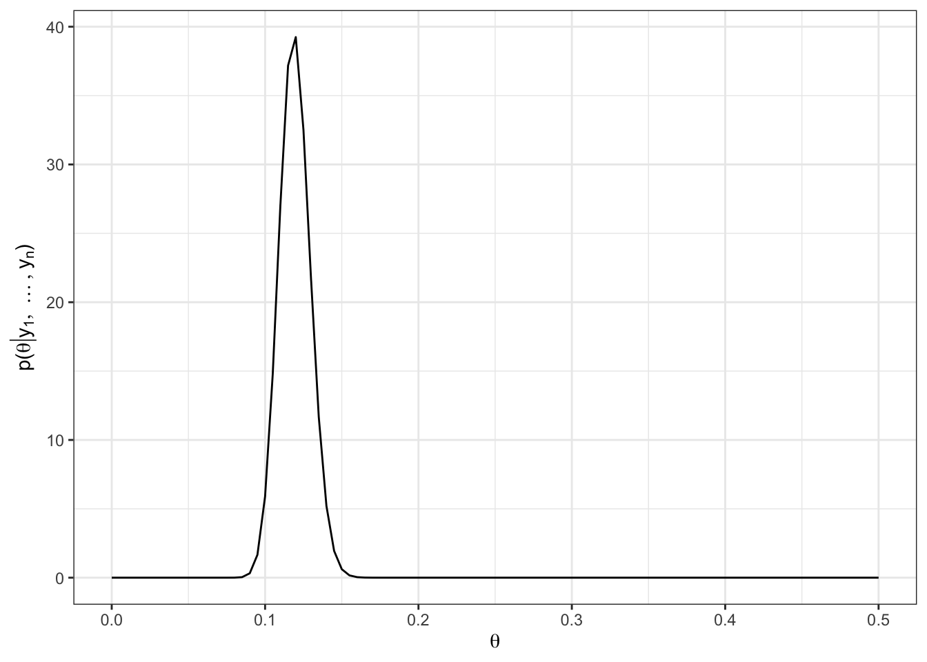
data.frame(x = c(0, 0.5)) %>%
ggplot(aes(x = x)) +
stat_function(fun = dgamma, args = list(shape = sumY + a,
rate = sumX + b)) +
labs(x = TeX("$\\theta$"), y = TeX("p($\\theta | y_1, \\ldots, y_n$)")) +
theme_bw()Given our prior of \(a = 9, b = 3\), \(E[\theta | y_1,\ldots, y_n] =\) 0.1194
Definition: a sufficient statistic is a function of the data \((y_1,\ldots y_n\)) that is sufficient to make inference about unknown parameters (\(\theta\)).
If density \(p(y|\theta)\) can be written \(h(y) c(\phi) e^{\phi t(y)}\) for some transform \(\phi = f(\theta)\) we can say \(p(y|\theta)\) belongs in the exponential family.
\(t(y)\) is referred to as the sufficient statistic.
If \(p(y|\theta)\) belongs in the exponential family, then the conjugate prior is \[ p(\phi | n_0, t_0) = \kappa(n_0, t_0)c(\phi)^{n_0} e^{n_0 t_0 \phi}, \] where \(\kappa(n_0, t_0)\) is a normalizing constant.
the conjugate prior is given over \(\phi\) and we’d have to transform back if we care about \(p(\theta)\).
\(n_0\) is interpreted as the prior sample size and \(t_0\) is the prior guess.
The resulting posterior is
\[ p(\phi | y_1,\ldots y_n) \propto p \left(\phi | n_0 + n, \frac{n_0 t_0 + n \sum t(y_i)/n}{n_0 + n}\right) \] In words, one can show that the kernel of the posterior of \(\phi\) is proportional to the kernel of the prior of \(\phi\) with specific parameters. Thereby, we have conjugacy.