[1] 0 1 0 0 0 0 0 0 0 0Is this a fair coin?
library(tidyverse)
library(latex2exp)
library(glue)
library(patchwork)

set.seed(3)
flips = rbinom(5000, size = 1, prob = 0.25)
flips %>% head(10)
We observe 10 flips from the same coin above, where 0 is “tails” and 1 is “heads”. In summary, we see Y = 1 heads in 10 coin flips. Is this a fair coin?
To articulate this mathematically, let \(\theta \in [0, 1]\) be the bias-weighting (the chance of heads) of the coin. Fundamentally, we want \(p(\theta | y)\), which we can expand via Bayes’ rule,
\[ p(\theta | y) = \frac{p(y|\theta) p(\theta)}{\int_{\theta \in \Theta} p(y|\theta) p(\theta) d\theta} \]
Label the following on the equation above: likelihood, prior, posterior, normalizing constant.
Likelihood: the data generative process. The joint probability (or density) of the data given the parameters of the model. Most often thought of as a function of the parameter. Note: not a density of the parameter.
Prior: Our a priori (beforehand) beliefs about the true population characteristics.
Posterior: Our a posteriori (afterwards) beliefs about the true population characteristics after having observed the data set \(y\).
Normalizing constant: A number that enables a pmf or pdf to integrate to 1.
Uniform prior
Let \(y\) be the number of heads in \(n\) coin flips.
\[ p(\theta | y) \propto \theta^{y}(1-\theta)^{n-y} \]
This is the kernel of a ___ density, where \(\alpha = y + 1\) and \(\beta = n - y + 1\), hence
\[ p(\theta | y) = \frac{\Gamma(n + 2)}{\Gamma(y + 1)\Gamma(n-y+1)} \theta^{y}(1-\theta)^{n-y} \]
and the posterior mean is \(\frac{y + 1}{n + 2}\) and the posterior variance is \(\frac{(y+1)(n - y + 1)}{(n + 2)^2 (n + 1)}\).
Let’s examine how the posterior evolves with each successive coin flip.
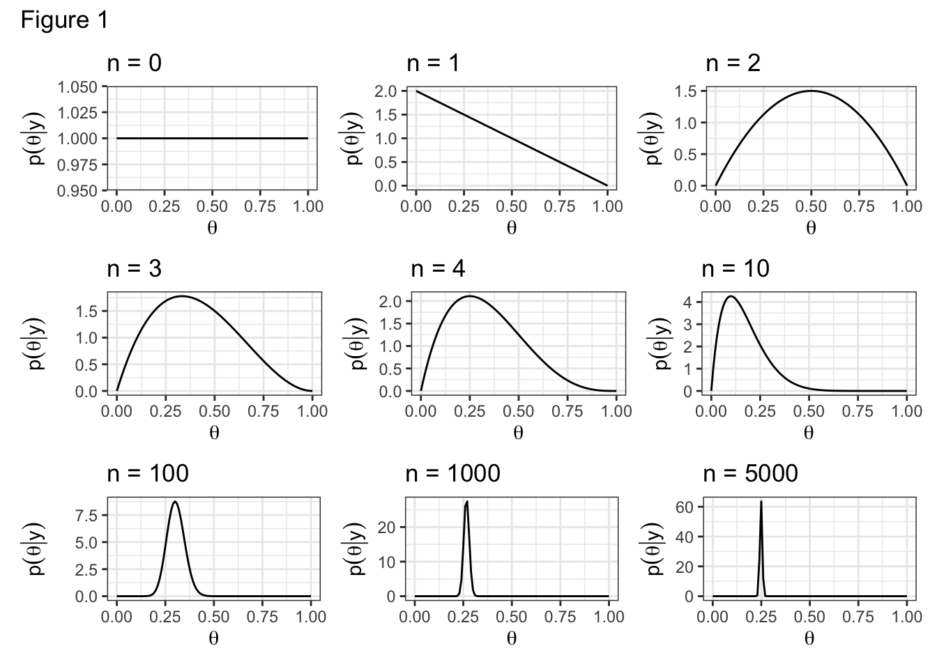
N = c(0, 1, 2, 3, 4, 10, 100, 1000, 5000)

for (i in seq_along(N)) {
n = N[i]
if(n == 0) {
  y = 0
}
else {
  y = sum(flips[1:n])
}

x = 0:1 # range
df = data.frame(x)
assign(paste0("p", i),
  df %>%
  ggplot(aes(x = x)) +
  stat_function(fun=dbeta,
                args = list(shape1 = y + 1, shape2 = n - y + 1)) +
  labs(y = TeX("$p(\\theta | y)$"), x = TeX("$\\theta$"),
       title = glue("n = {n}")) +
  theme_bw()
)
}

(p1 + p2 + p3) /
  (p4 + p5 + p6) /
  (p7 + p8 + p9) +
  plot_annotation(title = "Figure 1")
Conjugacy
If \(\theta \sim\) Uniform(0, 1) then \(p(\theta)\) = 1 for all \(\theta \in [0, 1]\).
Similarly, if \(\theta \sim\) beta(1, 1), then \(p(\theta) = 1\).
Claim:
If
\[ \begin{aligned} \theta &\sim \text{beta}(a, b)\\ Y | \theta &\sim \text{binomial}(n, \theta) \end{aligned} \] then
\[ p(\theta | Y) = \text{beta}(y + a, n - y + b) \]
Definition
A prior \(p(\theta)\) is said to be conjugate to the data generative model \(p(y|\theta)\) if the family of the posterior is necessarily in the same family as the prior. In math, \(p(\theta)\) is conjugate to \(p(y|\theta)\) if
\[ p(\theta) \in \mathcal{P} \implies p(\theta | y) \in \mathcal{P} \]
While conjugate priors make calculation easy, they may not accurately reflect our prior beliefs.
Prove the claim above.
Other priors
Incidentally, people are often satisfied with the choice of likelihood but are worried about the choice of prior.
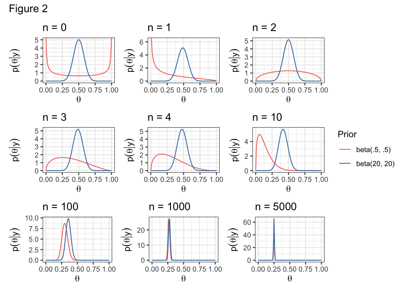
Let’s examine the effect of another couple of priors.
Given the coin’s dubious origin, we might believe a priori that the coin is biased. How could we represent this belief?
\[ \theta \sim \text{beta}(.5, .5) \]
Or alternatively, we might be strongly believe a priori that the coin is fair. How could we represent this belief?
\[ \theta \sim \text{beta}(20, 20) \]
How would you update the code of the previous example to show posterior inference under the prior \(\theta \sim\) beta(2,3)?
Prior data
In the example above, the parameters, a and b, of the conjugate prior are often thought of as prior data.
- a: “prior number of 1s”
- b: “prior number of 0s”
- a + b: “prior sample size”
We saw above that when a = 20 and b = 20, we needed more data to move the posterior.
Show that the posterior mean, \(E(\theta | y) = \frac{a + y}{a + b + n}\) converges to the sample average as \(n \rightarrow \infty\).