yTrain = readr::read_csv(
  "https://sta602-sp25.github.io/data/hw-digits-train.csv")

yTest = readr::read_csv(
  "https://sta602-sp25.github.io/data/hw-digits-test.csv"
)Homework 3
Due Friday February 7 at 5:00pm
Exercise 1
Let \(Y_1, \ldots Y_n | \theta\) be an i.i.d. random sample from a population with pdf \(p(y|\theta)\) where
\[ p(y|\theta) = \frac{2}{\Gamma(a)} \theta^{2a} y^{2a -1} e^{-\theta^2 y^2} \]
and \(y > 0\), \(\theta > 0\), \(a > 0\).
For this density,
\[ \begin{aligned} E~Y|\theta &= \frac{\Gamma(a + \frac{1}{2})}{\theta \Gamma(a)}\\ E~Y^2|\theta &= \frac{a}{\theta^2} \end{aligned} \]
Call this density \(g^2\) such that \(Y_1, \ldots Y_n | \theta \sim g^2(a, \theta)\).
Find the joint pdf of \(Y_1, \ldots Y_n | \theta\) and simplify as much as possible.
Suppose \(a\) is known but \(\theta\) is unknown. Identify a simple conjugate class of priors for \(\theta\). For any arbitrary member of the class, identify the posterior density \(p(\theta | y_1, \ldots y_n)\).
Obtain a formula for \(E~ \theta | Y_1, \ldots Y_n\) and \(Var~\theta | Y_1, \ldots Y_n\) when the prior is in the conjugate class.
Exercise 2
Handwritten digit classification. Data originally sourced from U.S. postal envelopes.
Exercise inspired by Prof. Hua Zhou’s Biostat M280.
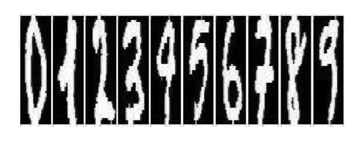
In this exercise, you will build a very simple Bayesian image classifier. Load the training and test data sets using the code below.
The training data set contains 3822 images like the ones displayed above. Each image is a 32 x 32 bitmap, i.e. 1024 pixels, where each pixel is either black (0) or white (1). The 1024 pixels are divided into 64 blocks of 4 x 4 pixels. Each digit in the data set is represented by a vector of these blocks \(\mathbf{x} = (x_1, \ldots, x_{64})\) where each element is a count of the white pixels in a block (a number between 0 and 16).
The 65th column of the data set (id) is the actual digit label.
How many of each digit are in the training data set? Create a histogram to show the distribution of
block10white pixels for each digit. What do you notice?Assume each digit (i.e. each
id) has its own multinomial data generative model. You can read about the multinomial distribution using?rmultinomin R.
Write down the joint density for images with id “j”, \(\prod_{k = 1}^{n_j} p(\mathbf{x}_k^{(j)} | \boldsymbol{\pi}^{(j)})\). Here \(n_j\) is the number of images of type \(j\) and \(\boldsymbol{\pi}^{(j)} = \{\pi_1^{(j)}, \ldots, \pi_{64}^{(j)} \}\)
How many total unknown parameters are in the complete joint density of all images?
Note
Notice that the multinomial sampling model places positive density on \(x_i > 16\), which is impossible in our data. This model is overly simple.
- The Dirichlet distribution is the multivariate generalization of the beta distribution. You can read more about it here. Place a Dirichlet prior on the probability parameters for each of your multinomial models in part b. Let the concentration parameters be all identically 1.
- Compute the posterior mean \(\hat{\boldsymbol{\pi}}^{(j)}\) for each \(j\) (or approximate it with Monte Carlo sampling). Hint: you may need to look up how to sample from a Dirichlet distribution in R. You may do this manually or find a package with built-in functions.
- For each image \(\mathbf{x}\) in your testing data set, compute your predicted id according to \(\text{argmax}_{j}~~p(\mathbf{x}| \boldsymbol{\hat{\pi}}^{(j)})p(j)\), where \(p(j)\) is the proportion of digit \(j\) in the training set. Report the number of correct and incorrect classifications in your testing data set.
Exercise 3
Suppose \(Y|\theta \sim \text{binary}(\theta)\) and we believe \(\theta \sim \text{Uniform}(0, 1)\) describes our uninformed prior beliefs about \(\theta\). However, we are really interested in the log-odds \(\gamma = f(\theta) = \log \frac{\theta}{1 - \theta}\).
Find the prior distribution for \(\gamma\) induced by our prior on \(\theta\). Is the prior informative about \(\gamma\)? Verify \(p(\gamma)\) using Monte Carlo sampling (i.e. sampling from \(p(\theta)\)) and then plotting the empirical density of the transformed samples along with the closed-form solution.
In general, is the mean of the transform the same as the transform of the mean? In other words, is \(E f(\theta) = f(E[\theta])\)? Why or why not? Hint: come up with another example.
Assume some data come in and \(\sum y_i = 7\) out of \(n = 10\) trials. Report the posterior mean and 95% posterior confidence interval for \(\gamma\). Is the transform of the quantile the quantile of the transform? Why or why not?